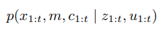
728x90

EKF SLAM

 확장 칼만필터 슬램은 가장 일찍 나온 슬램 알고리즘 중 하나로

최대 우도 데이터 연관을 사용한 온라인 슬램으라 할수 있습니다.


EKF SLAM의 가정들

1. 특징 기반 지도

 EKF SLAM에서 사용하는 지도는 점 특징 기반 지도가 사용되고,

여기서 점들의 갯수는 1000개 이하로 적으며, 점들 간에 구분하기 쉬울수록 잘 동작합니다.

EKF SLAM은 특징 검출기가 필요한데, 특징으로 인공 비콘이나 랜드마크를 사용합니다.


2. 가우시안 노이즈

 EKF SLAM은 로봇의 동작과 인지 시 가우시안 노이즈를 따른다고 가정하며

사후 확률의 불확실성은 상대적으로 작으나, EKF 선형화시 견딜수 없는 에러가 발생할 수 있습니다.


3. 긍정 측정치

 EKF SLAM은 랜드마크에 대한 긍정 정보만을 사용할수 있으며,

랜드마크가 사라지는 것같은 부정 정보를 처리할수 없습니다.


 EKF SLAM을 사용하는 경우 대응관계가 주어진 경우와 대응관계가 주어지지 않은 경우가 있으나

일반적으로 대응관계는 주어지지 않으며 파이썬 로보틱스에서 제공하는 예제 또한 그러하므로

이 경우에 대한 시뮬레이션 예제를 살펴보겠습니다.


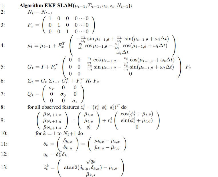
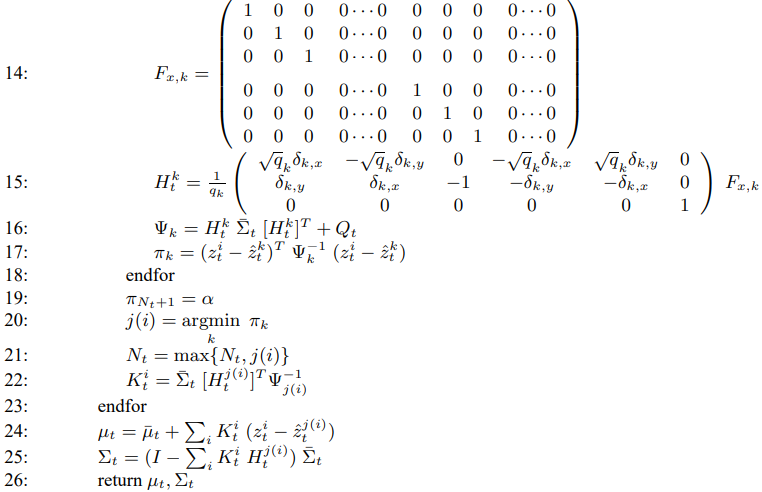
대응 관계가 주어지지 않은 EKF SLAM 알고리즘

 이 슬램 알고리즘은 대응 관계를 구하기 위해

증문 최대 우도 추정기 incremental maximum likelihood(ML)을 사용합니다.


import numpy as np
import math
import matplotlib.pyplot as plt


# EKF state covariance
Cx = np.diag([0.5, 0.5, math.radians(30.0)])**2

#  Simulation parameter
Qsim = np.diag([0.2, math.radians(1.0)])**2
Rsim = np.diag([1.0, math.radians(10.0)])**2

DT = 0.1  # time tick [s]
SIM_TIME = 60.0  # simulation time [s]
MAX_RANGE = 20.0  # maximum observation range
M_DIST_TH = 2.0  # Threshold of Mahalanobis distance for data association.
STATE_SIZE = 3  # State size [x,y,yaw]
LM_SIZE = 2  # LM srate size [x,y]

show_animation = True


늘 하던대로

임포트 라이브러리와 전역변수들을 살펴봅시다.


상태 공분산 Cx와 동작, 관측 노이즈 Q,Rsim을 초기화하고,

별도 파라미터들을 설정해 주었습니다.


def main():
    print(__file__ + " start!!")

    time = 0.0

    # RFID positions [x, y]
    RFID = np.array([[10.0, -2.0],
                     [15.0, 10.0],
                     [3.0, 15.0],
                     [-5.0, 20.0]])

    # State Vector [x y yaw v]'
    xEst = np.matrix(np.zeros((STATE_SIZE, 1)))
    xTrue = np.matrix(np.zeros((STATE_SIZE, 1)))
    PEst = np.eye(STATE_SIZE)

    xDR = np.matrix(np.zeros((STATE_SIZE, 1)))  # Dead reckoning

    # history
    hxEst = xEst
    hxTrue = xTrue
    hxDR = xTrue

    while SIM_TIME >= time:
        time += DT
        u = calc_input()

        xTrue, z, xDR, ud = observation(xTrue, xDR, u, RFID)

        xEst, PEst = ekf_slam(xEst, PEst, ud, z)

        x_state = xEst[0:STATE_SIZE]

        # store data history
        hxEst = np.hstack((hxEst, x_state))
        hxDR = np.hstack((hxDR, xDR))
        hxTrue = np.hstack((hxTrue, xTrue))

        if show_animation:
            plt.cla()

            plt.plot(RFID[:, 0], RFID[:, 1], "*k")
            plt.plot(xEst[0], xEst[1], ".r")

            # plot landmark
            for i in range(calc_n_LM(xEst)):
                plt.plot(xEst[STATE_SIZE + i * 2],
                         xEst[STATE_SIZE + i * 2 + 1], "xg")

            plt.plot(np.array(hxTrue[0, :]).flatten(),
                     np.array(hxTrue[1, :]).flatten(), "-b")
            plt.plot(np.array(hxDR[0, :]).flatten(),
                     np.array(hxDR[1, :]).flatten(), "-k")
            plt.plot(np.array(hxEst[0, :]).flatten(),
                     np.array(hxEst[1, :]).flatten(), "-r")
            plt.axis("equal")
            plt.grid(True)
            plt.pause(0.001)


if __name__ == '__main__':
    main()

 메인 함수를 보면, 플로팅 부분을 제외하고 루프 앞까지를 보면

랜드마크로 사용할 RFID 4개를 정의 하였습니다.


 이후 추정 상태 변수 xEst, 실제 상태 변수 xTrue

추정 상태 공분산 PEst를 만들어줍니다.

그 다음 추측항법도 비교해줄수 있도록 xDR도 만들고


 추측 항법 상태, 추정 상태, 실제 상태들을 담기위해

hx 변수들도 만들어 줍니다.

이제 루프문 내부를 확인하겠습니다.


    while SIM_TIME >= time:
        time += DT
        u = calc_input()

        xTrue, z, xDR, ud = observation(xTrue, xDR, u, RFID)

        xEst, PEst = ekf_slam(xEst, PEst, ud, z)

        x_state = xEst[0:STATE_SIZE]

        # store data history
        hxEst = np.hstack((hxEst, x_state))
        hxDR = np.hstack((hxDR, xDR))
        hxTrue = np.hstack((hxTrue, xTrue))

 맨 앞은 우리가 자주보던 입력 구하는 함수 calc_input

 그 다음에는 관측 함수

 ekf slam

 뒤에는 로봇의 상태변수들만 hx 변수에 담는 과정이 되겠습니다.


 calc input 함수는 입력값으로 사용할 선속도와 각속도를 반환하니 패스하고

 관측 함수 부터 살펴보겠습니다.


def observation(xTrue, xd, u, RFID):

    xTrue = motion_model(xTrue, u)

    # add noise to gps x-y
    z = np.matrix(np.zeros((0, 3)))

    for i in range(len(RFID[:, 0])):

        dx = RFID[i, 0] - xTrue[0, 0]
        dy = RFID[i, 1] - xTrue[1, 0]
        d = math.sqrt(dx**2 + dy**2)
        angle = pi_2_pi(math.atan2(dy, dx))
        if d <= MAX_RANGE:
            dn = d + np.random.randn() * Qsim[0, 0]  # add noise
            anglen = angle + np.random.randn() * Qsim[1, 1]  # add noise
            zi = np.matrix([dn, anglen, i])
            z = np.vstack((z, zi))

    # add noise to input
    ud1 = u[0, 0] + np.random.randn() * Rsim[0, 0]
    ud2 = u[1, 0] + np.random.randn() * Rsim[1, 1]
    ud = np.matrix([ud1, ud2]).T

    xd = motion_model(xd, ud)

    return xTrue, z, xd, ud

 관측 함수에서 처음에는 실제 로봇의 주행 궤적을 구하기 위해 xTrue를 동작시키고,

다음에는 관측치의 노이즈로 사용할 행렬을 생성 합니다.


 관측치인 거리와 방위는 실제 로봇의 위치와 랜드마크 사이의 거리로 구할수 있으므로

dx, dy를 통해 대각선 거리 d와 방위 angle을 구합니다.


 하지만 측정 가능 거리에 존재하는 랜드마크만 검출할수 있으므로 거리재한을 두고,

이 거리재한 안에 존재하는 랜드마크에 한해 가우시안 노이즈를 추가한 dn, anglen을 관측치 z로 추가합니다.


 다음으로 동작 모델을 사용하는데, 기존의 입력에 가우시안 노이즈를 추가하여

추측 항법 상태를 구합니다.


    while SIM_TIME >= time:
        time += DT
        u = calc_input()

        xTrue, z, xDR, ud = observation(xTrue, xDR, u, RFID)

        xEst, PEst = ekf_slam(xEst, PEst, ud, z)

        x_state = xEst[0:STATE_SIZE]

 관측 함수를 수행하였으니

다음으로 ekf slam 함수를 보겠습니다.


 여기서 이전 상태와 공분산, 노이즈가 추가된 입력,

관측 함수로 구한 관측치들이 매개변수로 사용됩니다.


def ekf_slam(xEst, PEst, u, z):

    # Predict
    S = STATE_SIZE
    xEst[0:S] = motion_model(xEst[0:S], u)
    G, Fx = jacob_motion(xEst[0:S], u)
    PEst[0:S, 0:S] = G.T * PEst[0:S, 0:S] * G + Fx.T * Cx * Fx
    initP = np.eye(2)

    # Update
    for iz in range(len(z[:, 0])):  # for each observation
        minid = search_correspond_LM_ID(xEst, PEst, z[iz, 0:2])

        nLM = calc_n_LM(xEst)
        if minid == nLM:
            print("New LM")
            # Extend state and covariance matrix
            xAug = np.vstack((xEst, calc_LM_Pos(xEst, z[iz, :])))
            PAug = np.vstack((np.hstack((PEst, np.zeros((len(xEst), LM_SIZE)))),
                              np.hstack((np.zeros((LM_SIZE, len(xEst))), initP))))
            xEst = xAug
            PEst = PAug

        lm = get_LM_Pos_from_state(xEst, minid)
        y, S, H = calc_innovation(lm, xEst, PEst, z[iz, 0:2], minid)

        K = PEst * H.T * np.linalg.inv(S)
        xEst = xEst + K * y
        PEst = (np.eye(len(xEst)) - K * H) * PEst

    xEst[2] = pi_2_pi(xEst[2])

    return xEst, PEst

 ekf slam 함수에서는 우선 예측 과정을 수행합니다.

여기서 추정할 상태는 x, y, yaw 이 3가지므로

추정 상태 공간으로부터 로봇의 자세 변수만 구하여 사용합니다.


 모션 모델 함수에 로봇의 이전 추정 자세와

노이즈 입력을 넣어 예측 추정치를 구하였습니다.


 다음 줄은 동작 모델의 자코비안을 구하는 것으로 잠시 살펴보겠습니다.


def jacob_motion(x, u):

    Fx = np.hstack((np.eye(STATE_SIZE), np.zeros(
        (STATE_SIZE, LM_SIZE * calc_n_LM(x)))))

    jF = np.matrix([[0.0, 0.0, -DT * u[0] * math.sin(x[2, 0])],
                    [0.0, 0.0, DT * u[0] * math.cos(x[2, 0])],
                    [0.0, 0.0, 0.0]])

    G = np.eye(STATE_SIZE) + Fx.T * jF * Fx

    return G, Fx,

 이 함수에는 동작 모델에서 구한 상태 변수들의

입력 변수에 대한 자코비안을 구한 결과를 반환합니다.


def ekf_slam(xEst, PEst, u, z):

    # Predict
    S = STATE_SIZE
    xEst[0:S] = motion_model(xEst[0:S], u)
    G, Fx = jacob_motion(xEst[0:S], u)
    PEst[0:S, 0:S] = G.T * PEst[0:S, 0:S] * G + Fx.T * Cx * Fx
    initP = np.eye(2)


 다시 ekf slam의 앞부분으로 돌아오면

방금 구한 자코비안을 통해 로봇의 추정 자세 변수들에 대한 예측 공분산을 구할수 있게 됩니다.

이 아래에는 관측치에 대한 루프를 돌리겠습니다.


    # Update
    for iz in range(len(z[:, 0])):  # for each observation
        minid = search_correspond_LM_ID(xEst, PEst, z[iz, 0:2])

        nLM = calc_n_LM(xEst)
        if minid == nLM:
            print("New LM")
            # Extend state and covariance matrix
            xAug = np.vstack((xEst, calc_LM_Pos(xEst, z[iz, :])))
            PAug = np.vstack((np.hstack((PEst, np.zeros((len(xEst), LM_SIZE)))),
                              np.hstack((np.zeros((LM_SIZE, len(xEst))), initP))))
            xEst = xAug
            PEst = PAug

        lm = get_LM_Pos_from_state(xEst, minid)
        y, S, H = calc_innovation(lm, xEst, PEst, z[iz, 0:2], minid)

        K = PEst * H.T * np.linalg.inv(S)
        xEst = xEst + K * y
        PEst = (np.eye(len(xEst)) - K * H) * PEst

    xEst[2] = pi_2_pi(xEst[2])

    return xEst, PEst


 이 루프문의 첫번째로

추정 상태와 추정 공분산, 관측이 주어질때 해당 랜드마크의 아이디를 찾는 함수입니다.


def search_correspond_LM_ID(xAug, PAug, zi):
    """
    Landmark association with Mahalanobis distance
    """

    nLM = calc_n_LM(xAug)

    mdist = []

    for i in range(nLM):
        lm = get_LM_Pos_from_state(xAug, i)
        y, S, H = calc_innovation(lm, xAug, PAug, zi, i)
        mdist.append(y.T * np.linalg.inv(S) * y)

    mdist.append(M_DIST_TH)  # new landmark

    minid = mdist.index(min(mdist))

    return minid


 이 랜드마크 아이디 탐색 함수는

마할라노비스 거리를 이용한 랜드마크 연관으로

매개변수로부터 전달받은 추정 상태를 통해 랜드마크의 갯수를 확인해 봅니다.


def calc_n_LM(x):
    n = int((len(x) - STATE_SIZE) / LM_SIZE)
    return n

 초기 추정 상태는 로봇의 자세 3개밖에 없지만

랜드마크가 검출 될수록 각 랜드마크의 위치 x, y 2개씩 추가 되게 됩니다.

그래서 전체 x의 길이 - 로봇 자세 3을 한 후 2를 나누어주면 그동안 관측한 랜드마크 갯수가 나오게 됩니다.


def search_correspond_LM_ID(xAug, PAug, zi):
    """
    Landmark association with Mahalanobis distance
    """

    nLM = calc_n_LM(xAug)

    mdist = []

    for i in range(nLM):
        lm = get_LM_Pos_from_state(xAug, i)
        y, S, H = calc_innovation(lm, xAug, PAug, zi, i)
        mdist.append(y.T * np.linalg.inv(S) * y)

    mdist.append(M_DIST_TH)  # new landmark

    minid = mdist.index(min(mdist))

    return minid


 추정 상태공간으로부터 랜드마크 갯수를 구한 후

마할라노비스 거리를 담을 텅빈 리스트를 만들어 주고

각 랜드마크에 대해 루프를 돌려봅시다.


    for i in range(nLM):
        lm = get_LM_Pos_from_state(xAug, i)
        y, S, H = calc_innovation(lm, xAug, PAug, zi, i)
        mdist.append(y.T * np.linalg.inv(S) * y)

    mdist.append(M_DIST_TH)  # new landmark

    minid = mdist.index(min(mdist))

    return minid

 가장 처음 만나는 함수는 추정 상태공간(로봇의 자세 + 랜드마크 위치들)에서

해당 랜드마크의 위치를 추출하는 함수가 됩니다.


def get_LM_Pos_from_state(x, ind):

    lm = x[STATE_SIZE + LM_SIZE * ind: STATE_SIZE + LM_SIZE * (ind + 1), :]

    return lm

 이 함수에서 해당 랜드마크를 찾아 랜드마크의 위치 (x, y)를 반환합니다.


    for i in range(nLM):
        lm = get_LM_Pos_from_state(xAug, i)
        y, S, H = calc_innovation(lm, xAug, PAug, zi, i)
        mdist.append(y.T * np.linalg.inv(S) * y)

    mdist.append(M_DIST_TH)  # new landmark

    minid = mdist.index(min(mdist))

    return minid


 랜드마크 위치, 추정 예측 상태, 추정 예측 공분산, 관측치, 랜드마크 인댁스를 이용해서

개변치 계산 calc_innovation 함수를 살펴보겠습니다.


def calc_innovation(lm, xEst, PEst, z, LMid):
    delta = lm - xEst[0:2]
    q = (delta.T * delta)[0, 0]
    zangle = math.atan2(delta[1], delta[0]) - xEst[2]
    zp = [math.sqrt(q), pi_2_pi(zangle)]
    y = (z - zp).T
    y[1] = pi_2_pi(y[1])
    H = jacobH(q, delta, xEst, LMid + 1)
    S = H * PEst * H.T + Cx[0:2, 0:2]

    return y, S, H


 개변치 계산 함수에서는 우선 랜드마크의 위치와 로봇의 자세 사이의 거리 delta를 계산하고,

delta의 제곱 q와 랜드마크와 로봇 사이 각인 zangle을 구합니다.


 이를 정리하여 예측 로봇 자세와 추정 랜드마크 사이 거리 + 각도로 이루어진 예측 zp를 구하고,

실제 관측치인 z에서 zp를 빼네어 실제 관측과 예측 관측사이의 차인 y를 구합니다.


 그 다음 거리 q와 예측 추정, 해당 랜드마크 번호로 관측에 대한 자코비안을 계산하는데

(jacobH 함수 생략) 자코비안 결과와 예측 추정 공분산 PEst, 그리고 노이즈 변수를 사용해

정리하면 실제 관측과 예측 관측사이 차 y, 자코비안 H, 계산한 분모 S를 반환합니다.


    for i in range(nLM):
        lm = get_LM_Pos_from_state(xAug, i)
        y, S, H = calc_innovation(lm, xAug, PAug, zi, i)
        mdist.append(y.T * np.linalg.inv(S) * y)

    mdist.append(M_DIST_TH)  # new landmark

    minid = mdist.index(min(mdist))

    return minid


개변치 계산 함수에서 돌아와

y와 S를 이용하여 마할라 노비스 거리를 계산하고,

마할라 노비스 거리 목록에 추가시켜줍니다.


 모든 랜드마크에 대한 마할라노비스 거리 목록이 만들어지면

마할라 노비스 거리 임계치도 추가해주고

그 중에 마할라노비스 거리가 가장 작은 값의 인덱스를 찾습니다.


 만약 마할라노비스거리 임계치의 인덱스가 나온다면

이는 새로운 랜드마크를 검출한 것이라 볼수 있겠습니다.


 아니면 다른 랜드마크에 대한 인덱스가 나온 경우

예측 추정 상태와 관측치로부터 가장 올바른 랜드마크를 찾은것이고

올바른 랜드마크의 아이디를 반환하게 됩니다.


def ekf_slam(xEst, PEst, u, z):

    # Predict
    S = STATE_SIZE
    xEst[0:S] = motion_model(xEst[0:S], u)
    G, Fx = jacob_motion(xEst[0:S], u)
    PEst[0:S, 0:S] = G.T * PEst[0:S, 0:S] * G + Fx.T * Cx * Fx
    initP = np.eye(2)

    # Update
    for iz in range(len(z[:, 0])):  # for each observation
        minid = search_correspond_LM_ID(xEst, PEst, z[iz, 0:2])

        nLM = calc_n_LM(xEst)
        if minid == nLM:
            print("New LM")
            # Extend state and covariance matrix
            xAug = np.vstack((xEst, calc_LM_Pos(xEst, z[iz, :])))
            PAug = np.vstack((np.hstack((PEst, np.zeros((len(xEst), LM_SIZE)))),
                              np.hstack((np.zeros((LM_SIZE, len(xEst))), initP))))
            xEst = xAug
            PEst = PAug

        lm = get_LM_Pos_from_state(xEst, minid)
        y, S, H = calc_innovation(lm, xEst, PEst, z[iz, 0:2], minid)

        K = PEst * H.T * np.linalg.inv(S)
        xEst = xEst + K * y
        PEst = (np.eye(len(xEst)) - K * H) * PEst

    xEst[2] = pi_2_pi(xEst[2])

    return xEst, PEst


 이재 랜드마크의 아이디를 찾는 함수를 완료하였으니 다시 내려가 봅시다.

랜드마크의 갯수를 세었는데, 반환받은 아이디와 같다면 새로운 랜드마크를 찾은게 됩니다.


 그래서 if 조건문 내부에

기존의 추정 상태 공간과 추정 공분산을 새 랜드마크에 대한 정보를 추가해 줍니다.


 예측 추정 상태와 랜드마크 아이디로 해당 랜드마크의 위치를 구하고,

개변치를 계산하고, 칼만 개인을 계산 후

예측 추정 상태에 칼만 개인과 실제 관측과 예측 관측사이 차 y를 더해주고,

예측 공분산에도 똑같이 반영을 해 줍니다.


 예측 추정 상태, 공분산에다가 모든 랜드마크에 대한 칼만게인, 관측차 등을 반영해주면

이 값은 실제 추정 상태값이라 할수 있습니다.

대응관계가 주어지지않은 경우 ekf slam를 살펴보았습니다.


 아래의 시뮬레이션에서

파란선 : 실제 궤적

검은 선 : 추측 항법 궤적

빨간선 : 확장 칼만 필터 추정 궤적

검은 점 : 랜드마크 실제 위치

녹색 x : 랜드마크 추정 위치


"""
Extended Kalman Filter SLAM example
author: Atsushi Sakai (@Atsushi_twi)
"""

import numpy as np
import math
import matplotlib.pyplot as plt


# EKF state covariance
Cx = np.diag([0.5, 0.5, math.radians(30.0)])**2

#  Simulation parameter
Qsim = np.diag([0.2, math.radians(1.0)])**2
Rsim = np.diag([1.0, math.radians(10.0)])**2

DT = 0.1  # time tick [s]
SIM_TIME = 60.0  # simulation time [s]
MAX_RANGE = 20.0  # maximum observation range
M_DIST_TH = 2.0  # Threshold of Mahalanobis distance for data association.
STATE_SIZE = 3  # State size [x,y,yaw]
LM_SIZE = 2  # LM srate size [x,y]

show_animation = True


def ekf_slam(xEst, PEst, u, z):

    # Predict
    S = STATE_SIZE
    xEst[0:S] = motion_model(xEst[0:S], u)
    G, Fx = jacob_motion(xEst[0:S], u)
    PEst[0:S, 0:S] = G.T * PEst[0:S, 0:S] * G + Fx.T * Cx * Fx
    initP = np.eye(2)

    # Update
    for iz in range(len(z[:, 0])):  # for each observation
        minid = search_correspond_LM_ID(xEst, PEst, z[iz, 0:2])

        nLM = calc_n_LM(xEst)
        if minid == nLM:
            print("New LM")
            # Extend state and covariance matrix
            xAug = np.vstack((xEst, calc_LM_Pos(xEst, z[iz, :])))
            PAug = np.vstack((np.hstack((PEst, np.zeros((len(xEst), LM_SIZE)))),
                              np.hstack((np.zeros((LM_SIZE, len(xEst))), initP))))
            xEst = xAug
            PEst = PAug

        lm = get_LM_Pos_from_state(xEst, minid)
        y, S, H = calc_innovation(lm, xEst, PEst, z[iz, 0:2], minid)
        K = PEst * H.T * np.linalg.inv(S)
        xEst = xEst + K * y
        PEst = (np.eye(len(xEst)) - K * H) * PEst

    xEst[2] = pi_2_pi(xEst[2])

    return xEst, PEst


def calc_input():
    v = 1.0  # [m/s]
    yawrate = 0.1  # [rad/s]
    u = np.matrix([v, yawrate]).T
    return u


def observation(xTrue, xd, u, RFID):

    xTrue = motion_model(xTrue, u)

    # add noise to gps x-y
    z = np.matrix(np.zeros((0, 3)))

    for i in range(len(RFID[:, 0])):

        dx = RFID[i, 0] - xTrue[0, 0]
        dy = RFID[i, 1] - xTrue[1, 0]
        d = math.sqrt(dx**2 + dy**2)
        angle = pi_2_pi(math.atan2(dy, dx))
        if d <= MAX_RANGE:
            dn = d + np.random.randn() * Qsim[0, 0]  # add noise
            anglen = angle + np.random.randn() * Qsim[1, 1]  # add noise
            zi = np.matrix([dn, anglen, i])
            z = np.vstack((z, zi))

    # add noise to input
    ud1 = u[0, 0] + np.random.randn() * Rsim[0, 0]
    ud2 = u[1, 0] + np.random.randn() * Rsim[1, 1]
    ud = np.matrix([ud1, ud2]).T

    xd = motion_model(xd, ud)

    return xTrue, z, xd, ud


def motion_model(x, u):

    F = np.matrix([[1.0, 0, 0],
                   [0, 1.0, 0],
                   [0, 0, 1.0]])

    B = np.matrix([[DT * math.cos(x[2, 0]), 0],
                   [DT * math.sin(x[2, 0]), 0],
                   [0.0, DT]])

    x = F * x + B * u

    return x


def calc_n_LM(x):
    n = int((len(x) - STATE_SIZE) / LM_SIZE)
    return n


def jacob_motion(x, u):

    Fx = np.hstack((np.eye(STATE_SIZE), np.zeros(
        (STATE_SIZE, LM_SIZE * calc_n_LM(x)))))

    jF = np.matrix([[0.0, 0.0, -DT * u[0] * math.sin(x[2, 0])],
                    [0.0, 0.0, DT * u[0] * math.cos(x[2, 0])],
                    [0.0, 0.0, 0.0]])

    G = np.eye(STATE_SIZE) + Fx.T * jF * Fx

    return G, Fx,


def calc_LM_Pos(x, z):

    zp = np.zeros((2, 1))

    zp[0, 0] = x[0, 0] + z[0, 0] * math.cos(x[2, 0] + z[0, 1])
    zp[1, 0] = x[1, 0] + z[0, 0] * math.sin(x[2, 0] + z[0, 1])

    return zp


def get_LM_Pos_from_state(x, ind):

    lm = x[STATE_SIZE + LM_SIZE * ind: STATE_SIZE + LM_SIZE * (ind + 1), :]

    return lm


def search_correspond_LM_ID(xAug, PAug, zi):
    """
    Landmark association with Mahalanobis distance
    """

    nLM = calc_n_LM(xAug)

    mdist = []

    for i in range(nLM):
        lm = get_LM_Pos_from_state(xAug, i)
        y, S, H = calc_innovation(lm, xAug, PAug, zi, i)
        mdist.append(y.T * np.linalg.inv(S) * y)

    mdist.append(M_DIST_TH)  # new landmark

    minid = mdist.index(min(mdist))

    return minid


def calc_innovation(lm, xEst, PEst, z, LMid):
    delta = lm - xEst[0:2]
    q = (delta.T * delta)[0, 0]
    zangle = math.atan2(delta[1], delta[0]) - xEst[2]
    zp = [math.sqrt(q), pi_2_pi(zangle)]
    y = (z - zp).T
    y[1] = pi_2_pi(y[1])
    H = jacobH(q, delta, xEst, LMid + 1)
    S = H * PEst * H.T + Cx[0:2, 0:2]
    #H = np.array(H, dtype=np.float)
    return y, S, H


def jacobH(q, delta, x, i):
    sq = math.sqrt(q)
    G = np.matrix([[-sq * delta[0, 0], - sq * delta[1, 0], 0, sq * delta[0, 0], sq * delta[1, 0]],
                   [delta[1, 0], - delta[0, 0], - 1.0, - delta[1, 0], delta[0, 0]]])
    G = G / q
    nLM = calc_n_LM(x)
    F1 = np.hstack((np.eye(3), np.zeros((3, 2 * nLM))))
    F2 = np.hstack((np.zeros((2, 3)), np.zeros((2, 2 * (i - 1))),
                    np.eye(2), np.zeros((2, 2 * nLM - 2 * i))))

    F = np.vstack((F1, F2))
    H = G * F

    return H


def pi_2_pi(angle):
    return float((angle + math.pi) % (2*math.pi) - math.pi)


def main():
    print(__file__ + " start!!")

    time = 0.0

    # RFID positions [x, y]
    RFID = np.array([[10.0, -2.0],
                     [15.0, 10.0],
                     [3.0, 15.0],
                     [-5.0, 20.0]])

    # State Vector [x y yaw v]'
    xEst = np.matrix(np.zeros((STATE_SIZE, 1)))
    xTrue = np.matrix(np.zeros((STATE_SIZE, 1)))
    PEst = np.eye(STATE_SIZE)

    xDR = np.matrix(np.zeros((STATE_SIZE, 1)))  # Dead reckoning

    # history
    hxEst = xEst
    hxTrue = xTrue
    hxDR = xTrue

    while SIM_TIME >= time:
        time += DT
        u = calc_input()

        xTrue, z, xDR, ud = observation(xTrue, xDR, u, RFID)

        xEst, PEst = ekf_slam(xEst, PEst, ud, z)

        x_state = xEst[0:STATE_SIZE]

        # store data history
        hxEst = np.hstack((hxEst, x_state))
        hxDR = np.hstack((hxDR, xDR))
        hxTrue = np.hstack((hxTrue, xTrue))

        if show_animation:
            plt.cla()

            plt.plot(RFID[:, 0], RFID[:, 1], "*k")
            plt.plot(xEst[0], xEst[1], ".r")

            # plot landmark
            for i in range(calc_n_LM(xEst)):
                plt.plot(xEst[STATE_SIZE + i * 2],
                         xEst[STATE_SIZE + i * 2 + 1], "xg")

            plt.plot(np.array(hxTrue[0, :]).flatten(),
                     np.array(hxTrue[1, :]).flatten(), "-b")
            plt.plot(np.array(hxDR[0, :]).flatten(),
                     np.array(hxDR[1, :]).flatten(), "-k")
            plt.plot(np.array(hxEst[0, :]).flatten(),
                     np.array(hxEst[1, :]).flatten(), "-r")
            plt.axis("equal")
            plt.grid(True)
            plt.pause(0.001)


if __name__ == '__main__':
    main()
300x250
728x90

SLAM이란?

 SLAM은 Simultaneous Localization and Mapping의 약어로 로봇 공학에서 주요한 분야 중

하나인 로봇의 동시적인 위치 추정과 지도 작성에 대한 문제를 말합니다.


SLAM의 필요성

 일반적인 경우 로봇은 주변 환경에 대한 정보, 즉 지도를 가지고 있지 않으며

그러한 공간에서 자신의 위치를 인지할 필요가 있습니다.

 이 문제를 해결하기 위해 지도를 작성하고, 작성된 지도를 기반으로

자신이 어디에 있는지 추정하는 것이 필요하게 되었습니다.


SLAM의 종류

 슬램 문제 종류로 2가지가 있습니다.

1. 온라인 슬램 online slam problem

 온라인 슬램은 제어 입력과 관측치들이 주어질때 지도와 로봇의 순간적인 위치를 추정하는 문제 입니다. 

많은 온라인 슬램 알고리즘은 시간이 지남에 따라 이전의 관측치와 제어 입력을 버리게 됩니다.

2. 완전 슬램 full slam ploblem

 완전 슬램은 온라인 슬램과 달리 지도와 로봇의 전체 경로를 추정하는 문제입니다.


완전 슬램으로 온라인 슬램 구하기

 온라인 슬램은 완전 슬램의 이전 자세들을 적분한 결과로 구할수 있으며,

매 시간마다 이러한 적분이 수행되어 로봇의 현재 위치를 구하게 됩니다.


슬램과 추정

 슬램은 근본적으로 연속 요소와 이산 요소를 추정하는 문제라 할수 있습니다.

1. 연속 요소

  슬램에서 추정해야할 연속 공간 요소로 지도 상에 존재하는 물체의 위치와

로봇의 자세 변수가 있습니다.

2. 이산 요소

 슬램에서 추정을 해야하는 이산 공간 요소로 대응 관계가 있습니다.

여기서 대응관계란 슬램 알고리즘이 현재 찾은 물체가 이전에 찾은 물체인지

관계를 찾아내는것을 말합니다.


슬램과 대응관계

 대응 관계를 다루는 온라인 슬램의 사후확률은 아래와 같습니다.

 완전 슬램의 경우는 다음과 같습니다.

 온라인 슬램 사후확률은 완전 슬램의 이전 자세들을 적분하고,

이전 시간들의 대응관계를 합하여 구할 수 있습니다.


완전 슬램의 한계

 온라인 슬램과 완전 슬램은 슬램 문제의 표준이라 할수 있으나

완전 슬램 사후확률은 모든 변수들을 계산하여야 하므로 다음의 두가지 이유로 불가능 합니다.

(1) 연속 공간이 매우 크며, (2) 이산 대응관계 변수들도 많습니다.


슬램 문제에서 대응관계 변수 근사화의 필요성

 수 많은 슬램알고리즘들은 수만개 혹은 그이상의 특징들을 다루며,

대응 관계가 알려진 경우라 해도 계산해야할 양이 아주 많습니다.

 하지만 일반적인 경우 대응관계를 알수 없으므로,

모든 대응관계 변수의 백터는 시간에 따라 지수적으로 증가하게 됩니다.

즉, 실제 슬램 알고리즘을 사용할 때는 대응 관계를 다루기 위해 근사화가 필요합니다.


300x250
728x90

 파이썬 로보틱스를 통해 위치 추정과 지도 작성 알고리즘들의 종류와

이에 관련한 이론적인 내용들을 살펴보고

각 알고리즘들의 시뮬레이션 결과를 확인하였습니다.


 이 다음으로 확률적 로봇공학을 이용한 핵심 문제인 SLAM에 대해서 살펴보려고 합니다.

파이썬 로보틱스에서 제공하는 슬램 시뮬레이션의 예시로


1. EKF SLAM

2. FastSLAM 1

3. FastSLAM 2

4. GraphBasedSLAM

5. iterative_closets_point icp


5가지에 대해서 제공하고 있습니다.


 이번 SLAM 문제들도 필요한 이론적인 내용과 함께 같이 살펴보겠습니다.


300x250
728x90

 이번에는 라이다 스캔 데이터를 가지고 

격자 지도를 작성하는 예제를 다뤄보겠습니다.


 우선 임포트 라이브러리와 파라미터를 잠깐 살펴보겠습니다.


import math
from collections import deque

import matplotlib.pyplot as plt
import numpy as np

EXTEND_AREA = 1.0

별 내용없으니 바로

main 문으로 갑시다


def main():
    """
    Example usage
    """
    print(__file__, "start")
    xy_resolution = 0.02  # x-y grid resolution
    ang, dist = file_read("lidar01.csv")
    ox = np.sin(ang) * dist
    oy = np.cos(ang) * dist
    occupancy_map, min_x, max_x, min_y, max_y, xy_resolution = \
        generate_ray_casting_grid_map(ox, oy, xy_resolution, True)
    xy_res = np.array(occupancy_map).shape
    plt.figure(1, figsize=(10, 4))
    plt.subplot(122)
    plt.imshow(occupancy_map, cmap="PiYG_r")
    # cmap = "binary" "PiYG_r" "PiYG_r" "bone" "bone_r" "RdYlGn_r"
    plt.clim(-0.4, 1.4)
    plt.gca().set_xticks(np.arange(-.5, xy_res[1], 1), minor=True)
    plt.gca().set_yticks(np.arange(-.5, xy_res[0], 1), minor=True)
    plt.grid(True, which="minor", color="w", linewidth=0.6, alpha=0.5)
    plt.colorbar()
    plt.subplot(121)
    plt.plot([oy, np.zeros(np.size(oy))], [ox, np.zeros(np.size(oy))], "ro-")
    plt.axis("equal")
    plt.plot(0.0, 0.0, "ob")
    plt.gca().set_aspect("equal", "box")
    bottom, top = plt.ylim()  # return the current y-lim
    plt.ylim((top, bottom))  # rescale y axis, to match the grid orientation
    plt.grid(True)
    plt.show()


if __name__ == '__main__':
    main()

격자 해상도는 0.02

'lidar01.csv'파일을 읽어 각도와 거리값 행렬을 얻고

각 점들의 x, y 좌표를 구합니다. ox, oy

그 다음 광선 투사 그리드 맵 생성 함수 호출하고

뒷 부분에는 점유 격자지도와 데이터를 시각화 하는 코드가 되겠습니다.


그러면 광선투사 격자 지도 작성 함수를 보겠습니다.


def generate_ray_casting_grid_map(ox, oy, xy_resolution, breshen=True):
    """
    The breshen boolean tells if it's computed with bresenham ray casting
    (True) or with flood fill (False)
    """
    min_x, min_y, max_x, max_y, x_w, y_w = calc_grid_map_config(
        ox, oy, xy_resolution)
    # default 0.5 -- [[0.5 for i in range(y_w)] for i in range(x_w)]
    occupancy_map = np.ones((x_w, y_w)) / 2
    center_x = int(
        round(-min_x / xy_resolution))  # center x coordinate of the grid map
    center_y = int(
        round(-min_y / xy_resolution))  # center y coordinate of the grid map
    # occupancy grid computed with bresenham ray casting
    if breshen:
        for (x, y) in zip(ox, oy):
            # x coordinate of the the occupied area
            ix = int(round((x - min_x) / xy_resolution))
            # y coordinate of the the occupied area
            iy = int(round((y - min_y) / xy_resolution))
            laser_beams = bresenham((center_x, center_y), (
                ix, iy))  # line form the lidar to the occupied point
            for laser_beam in laser_beams:
                occupancy_map[laser_beam[0]][
                    laser_beam[1]] = 0.0  # free area 0.0
            occupancy_map[ix][iy] = 1.0  # occupied area 1.0
            occupancy_map[ix + 1][iy] = 1.0  # extend the occupied area
            occupancy_map[ix][iy + 1] = 1.0  # extend the occupied area
            occupancy_map[ix + 1][iy + 1] = 1.0  # extend the occupied area
    # occupancy grid computed with with flood fill
    else:
        occupancy_map = init_flood_fill((center_x, center_y), (ox, oy),
                                        (x_w, y_w),
                                        (min_x, min_y), xy_resolution)
        flood_fill((center_x, center_y), occupancy_map)
        occupancy_map = np.array(occupancy_map, dtype=np.float)
        for (x, y) in zip(ox, oy):
            ix = int(round((x - min_x) / xy_resolution))
            iy = int(round((y - min_y) / xy_resolution))
            occupancy_map[ix][iy] = 1.0  # occupied area 1.0
            occupancy_map[ix + 1][iy] = 1.0  # extend the occupied area
            occupancy_map[ix][iy + 1] = 1.0  # extend the occupied area
            occupancy_map[ix + 1][iy + 1] = 1.0  # extend the occupied area
    return occupancy_map, min_x, max_x, min_y, max_y, xy_resolution

 이 함수를 보니 격자 지도 생성방법중에

breshen 광선투사와 홍수 알고리즘을 사용하는 두가지가 있나 봅니다.

우리는 광선투사 방법을 다룰것이니 일단 처음부터 내려가봅시다.


 격자 지도 설정 계산 함수로 최대 최소 길이와 격자 갯수를 구하고

모든 값이 0.5인 점유 격자를 생성합니다.

다음 점유 격자 지도의 중시 값을 찾은뒤, 브레즌햄 광선 투사로 점유 격자 계산을 시작합니다.


* 브레슨햄

브레즌햄(Bresenham) 알고리즘 브레즌햄 알고리즘은 컴퓨터 그래픽스에서 복잡하고 계산을 느리게 만드는 실수 계산을 배제하고 정수 계산만으로 직선을 그리기 위해 만들어진 알고리즘 입니다

 - kukuta.tistory.com/186


        for (x, y) in zip(ox, oy):
            # x coordinate of the the occupied area
            ix = int(round((x - min_x) / xy_resolution))
            # y coordinate of the the occupied area
            iy = int(round((y - min_y) / xy_resolution))
            laser_beams = bresenham((center_x, center_y), (
                ix, iy))  # line form the lidar to the occupied point
            for laser_beam in laser_beams:
                occupancy_map[laser_beam[0]][
                    laser_beam[1]] = 0.0  # free area 0.0
            occupancy_map[ix][iy] = 1.0  # occupied area 1.0
            occupancy_map[ix + 1][iy] = 1.0  # extend the occupied area
            occupancy_map[ix][iy + 1] = 1.0  # extend the occupied area
            occupancy_map[ix + 1][iy + 1] = 1.0  # extend the occupied area

 브래즌햄 광선투사를 사용하는 경우 일단 모든 관측치에 대한 x, y 값을 각각 반복시킵니다.

해당 좌표에 존재하는 격자 인덱스 ix, iy를 구한뒤

브래즌햄 함수로 레이저 빔을 구합니다.


def bresenham(start, end):
    """
    Implementation of Bresenham's line drawing algorithm
    See en.wikipedia.org/wiki/Bresenham's_line_algorithm
    Bresenham's Line Algorithm
    Produces a np.array from start and end (original from roguebasin.com)
    >>> points1 = bresenham((4, 4), (6, 10))
    >>> print(points1)
    np.array([[4,4], [4,5], [5,6], [5,7], [5,8], [6,9], [6,10]])
    """
    # setup initial conditions
    x1, y1 = start
    x2, y2 = end
    dx = x2 - x1
    dy = y2 - y1
    is_steep = abs(dy) > abs(dx)  # determine how steep the line is
    if is_steep:  # rotate line
        x1, y1 = y1, x1
        x2, y2 = y2, x2
    # swap start and end points if necessary and store swap state
    swapped = False
    if x1 > x2:
        x1, x2 = x2, x1
        y1, y2 = y2, y1
        swapped = True
    dx = x2 - x1  # recalculate differentials
    dy = y2 - y1  # recalculate differentials
    error = int(dx / 2.0)  # calculate error
    y_step = 1 if y1 < y2 else -1
    # iterate over bounding box generating points between start and end
    y = y1
    points = []
    for x in range(x1, x2 + 1):
        coord = [y, x] if is_steep else (x, y)
        points.append(coord)
        error -= abs(dy)
        if error < 0:
            y += y_step
            error += dx
    if swapped:  # reverse the list if the coordinates were swapped
        points.reverse()
    points = np.array(points)
    return points


 브레즈햄 광선 투사 알고리즘을 통해 해당 광선이 지나가는 격자들의 좌표 목록을 구하게 됩니다.


* 브레즈햄 직선 알고리즘 예시

(0,0)은 그리드 왼쪽 위 구석, (1,1) 선의 왼쪽 맨위, (11, 5) 선의 오른쪽 바닥

        for (x, y) in zip(ox, oy):
            # x coordinate of the the occupied area
            ix = int(round((x - min_x) / xy_resolution))
            # y coordinate of the the occupied area
            iy = int(round((y - min_y) / xy_resolution))
            laser_beams = bresenham((center_x, center_y), (
                ix, iy))  # line form the lidar to the occupied point
            for laser_beam in laser_beams:
                occupancy_map[laser_beam[0]][
                    laser_beam[1]] = 0.0  # free area 0.0
            occupancy_map[ix][iy] = 1.0  # occupied area 1.0
            occupancy_map[ix + 1][iy] = 1.0  # extend the occupied area
            occupancy_map[ix][iy + 1] = 1.0  # extend the occupied area
            occupancy_map[ix + 1][iy + 1] = 1.0  # extend the occupied area

 광선 투사가 지나가는 격자 목록들을 laser_beams로 받아

모든 값들을 텅빈 공간이므로(레이저가 지나가니) 0.0으로 지정하고

빔이 도달한 지점을 점유된 공간이므로 1로 지정해줍니다.


def generate_ray_casting_grid_map(ox, oy, xy_resolution, breshen=True):
    """
    The breshen boolean tells if it's computed with bresenham ray casting
    (True) or with flood fill (False)
    """
    min_x, min_y, max_x, max_y, x_w, y_w = calc_grid_map_config(
        ox, oy, xy_resolution)
    # default 0.5 -- [[0.5 for i in range(y_w)] for i in range(x_w)]
    occupancy_map = np.ones((x_w, y_w)) / 2
    center_x = int(
        round(-min_x / xy_resolution))  # center x coordinate of the grid map
    center_y = int(
        round(-min_y / xy_resolution))  # center y coordinate of the grid map
    # occupancy grid computed with bresenham ray casting
    if breshen:
        for (x, y) in zip(ox, oy):
            # x coordinate of the the occupied area
            ix = int(round((x - min_x) / xy_resolution))
            # y coordinate of the the occupied area
            iy = int(round((y - min_y) / xy_resolution))
            laser_beams = bresenham((center_x, center_y), (
                ix, iy))  # line form the lidar to the occupied point
            for laser_beam in laser_beams:
                occupancy_map[laser_beam[0]][
                    laser_beam[1]] = 0.0  # free area 0.0
            occupancy_map[ix][iy] = 1.0  # occupied area 1.0
            occupancy_map[ix + 1][iy] = 1.0  # extend the occupied area
            occupancy_map[ix][iy + 1] = 1.0  # extend the occupied area
            occupancy_map[ix + 1][iy + 1] = 1.0  # extend the occupied area
    # occupancy grid computed with with flood fill
    else:
        occupancy_map = init_flood_fill((center_x, center_y), (ox, oy),
                                        (x_w, y_w),
                                        (min_x, min_y), xy_resolution)
        flood_fill((center_x, center_y), occupancy_map)
        occupancy_map = np.array(occupancy_map, dtype=np.float)
        for (x, y) in zip(ox, oy):
            ix = int(round((x - min_x) / xy_resolution))
            iy = int(round((y - min_y) / xy_resolution))
            occupancy_map[ix][iy] = 1.0  # occupied area 1.0
            occupancy_map[ix + 1][iy] = 1.0  # extend the occupied area
            occupancy_map[ix][iy + 1] = 1.0  # extend the occupied area
            occupancy_map[ix + 1][iy + 1] = 1.0  # extend the occupied area
    return occupancy_map, min_x, max_x, min_y, max_y, xy_resolution

 이렇게 계산된 점유 격자와 지도 크기, 해상도 등의 정보가 메인함수로 반환됩니다.


    xy_res = np.array(occupancy_map).shape
    plt.figure(1, figsize=(10, 4))
    plt.subplot(122)
    plt.imshow(occupancy_map, cmap="PiYG_r")
    # cmap = "binary" "PiYG_r" "PiYG_r" "bone" "bone_r" "RdYlGn_r"
    plt.clim(-0.4, 1.4)
    plt.gca().set_xticks(np.arange(-.5, xy_res[1], 1), minor=True)
    plt.gca().set_yticks(np.arange(-.5, xy_res[0], 1), minor=True)
    plt.grid(True, which="minor", color="w", linewidth=0.6, alpha=0.5)
    plt.colorbar()
    plt.subplot(121)
    plt.plot([oy, np.zeros(np.size(oy))], [ox, np.zeros(np.size(oy))], "ro-")
    plt.axis("equal")
    plt.plot(0.0, 0.0, "ob")
    plt.gca().set_aspect("equal", "box")
    bottom, top = plt.ylim()  # return the current y-lim
    plt.ylim((top, bottom))  # rescale y axis, to match the grid orientation
    plt.grid(True)
    plt.show()

 메인 함수의 플롯 부분을 살펴보면

우측에 점유 격자 지도를 놓고 좌측에는 레이저 빔 결과를 보여주고 있습니다.

이런 식으로 플로팅한 결과는 아래와 같습니다.


전체 코드

"""
LIDAR to 2D grid map example
author: Erno Horvath, Csaba Hajdu based on Atsushi Sakai's scripts
"""

import math
from collections import deque

import matplotlib.pyplot as plt
import numpy as np

EXTEND_AREA = 1.0


def file_read(f):
    """
    Reading LIDAR laser beams (angles and corresponding distance data)
    """
    with open(f) as data:
        measures = [line.split(",") for line in data]
    angles = []
    distances = []
    for measure in measures:
        angles.append(float(measure[0]))
        distances.append(float(measure[1]))
    angles = np.array(angles)
    distances = np.array(distances)
    return angles, distances


def bresenham(start, end):
    """
    Implementation of Bresenham's line drawing algorithm
    See en.wikipedia.org/wiki/Bresenham's_line_algorithm
    Bresenham's Line Algorithm
    Produces a np.array from start and end (original from roguebasin.com)
    >>> points1 = bresenham((4, 4), (6, 10))
    >>> print(points1)
    np.array([[4,4], [4,5], [5,6], [5,7], [5,8], [6,9], [6,10]])
    """
    # setup initial conditions
    x1, y1 = start
    x2, y2 = end
    dx = x2 - x1
    dy = y2 - y1
    is_steep = abs(dy) > abs(dx)  # determine how steep the line is
    if is_steep:  # rotate line
        x1, y1 = y1, x1
        x2, y2 = y2, x2
    # swap start and end points if necessary and store swap state
    swapped = False
    if x1 > x2:
        x1, x2 = x2, x1
        y1, y2 = y2, y1
        swapped = True
    dx = x2 - x1  # recalculate differentials
    dy = y2 - y1  # recalculate differentials
    error = int(dx / 2.0)  # calculate error
    y_step = 1 if y1 < y2 else -1
    # iterate over bounding box generating points between start and end
    y = y1
    points = []
    for x in range(x1, x2 + 1):
        coord = [y, x] if is_steep else (x, y)
        points.append(coord)
        error -= abs(dy)
        if error < 0:
            y += y_step
            error += dx
    if swapped:  # reverse the list if the coordinates were swapped
        points.reverse()
    points = np.array(points)
    return points


def calc_grid_map_config(ox, oy, xy_resolution):
    """
    Calculates the size, and the maximum distances according to the the
    measurement center
    """
    min_x = round(min(ox) - EXTEND_AREA / 2.0)
    min_y = round(min(oy) - EXTEND_AREA / 2.0)
    max_x = round(max(ox) + EXTEND_AREA / 2.0)
    max_y = round(max(oy) + EXTEND_AREA / 2.0)
    xw = int(round((max_x - min_x) / xy_resolution))
    yw = int(round((max_y - min_y) / xy_resolution))
    print("The grid map is ", xw, "x", yw, ".")
    return min_x, min_y, max_x, max_y, xw, yw


def atan_zero_to_twopi(y, x):
    angle = math.atan2(y, x)
    if angle < 0.0:
        angle += math.pi * 2.0
    return angle


def init_flood_fill(center_point, obstacle_points, xy_points, min_coord,
                    xy_resolution):
    """
    center_point: center point
    obstacle_points: detected obstacles points (x,y)
    xy_points: (x,y) point pairs
    """
    center_x, center_y = center_point
    prev_ix, prev_iy = center_x - 1, center_y
    ox, oy = obstacle_points
    xw, yw = xy_points
    min_x, min_y = min_coord
    occupancy_map = (np.ones((xw, yw))) * 0.5
    for (x, y) in zip(ox, oy):
        # x coordinate of the the occupied area
        ix = int(round((x - min_x) / xy_resolution))
        # y coordinate of the the occupied area
        iy = int(round((y - min_y) / xy_resolution))
        free_area = bresenham((prev_ix, prev_iy), (ix, iy))
        for fa in free_area:
            occupancy_map[fa[0]][fa[1]] = 0  # free area 0.0
        prev_ix = ix
        prev_iy = iy
    return occupancy_map


def flood_fill(center_point, occupancy_map):
    """
    center_point: starting point (x,y) of fill
    occupancy_map: occupancy map generated from Bresenham ray-tracing
    """
    # Fill empty areas with queue method
    sx, sy = occupancy_map.shape
    fringe = deque()
    fringe.appendleft(center_point)
    while fringe:
        n = fringe.pop()
        nx, ny = n
        # West
        if nx > 0:
            if occupancy_map[nx - 1, ny] == 0.5:
                occupancy_map[nx - 1, ny] = 0.0
                fringe.appendleft((nx - 1, ny))
        # East
        if nx < sx - 1:
            if occupancy_map[nx + 1, ny] == 0.5:
                occupancy_map[nx + 1, ny] = 0.0
                fringe.appendleft((nx + 1, ny))
        # North
        if ny > 0:
            if occupancy_map[nx, ny - 1] == 0.5:
                occupancy_map[nx, ny - 1] = 0.0
                fringe.appendleft((nx, ny - 1))
        # South
        if ny < sy - 1:
            if occupancy_map[nx, ny + 1] == 0.5:
                occupancy_map[nx, ny + 1] = 0.0
                fringe.appendleft((nx, ny + 1))


def generate_ray_casting_grid_map(ox, oy, xy_resolution, breshen=True):
    """
    The breshen boolean tells if it's computed with bresenham ray casting
    (True) or with flood fill (False)
    """
    min_x, min_y, max_x, max_y, x_w, y_w = calc_grid_map_config(
        ox, oy, xy_resolution)
    # default 0.5 -- [[0.5 for i in range(y_w)] for i in range(x_w)]
    occupancy_map = np.ones((x_w, y_w)) / 2
    center_x = int(
        round(-min_x / xy_resolution))  # center x coordinate of the grid map
    center_y = int(
        round(-min_y / xy_resolution))  # center y coordinate of the grid map
    # occupancy grid computed with bresenham ray casting
    if breshen:
        for (x, y) in zip(ox, oy):
            # x coordinate of the the occupied area
            ix = int(round((x - min_x) / xy_resolution))
            # y coordinate of the the occupied area
            iy = int(round((y - min_y) / xy_resolution))
            laser_beams = bresenham((center_x, center_y), (
                ix, iy))  # line form the lidar to the occupied point
            for laser_beam in laser_beams:
                occupancy_map[laser_beam[0]][
                    laser_beam[1]] = 0.0  # free area 0.0
            occupancy_map[ix][iy] = 1.0  # occupied area 1.0
            occupancy_map[ix + 1][iy] = 1.0  # extend the occupied area
            occupancy_map[ix][iy + 1] = 1.0  # extend the occupied area
            occupancy_map[ix + 1][iy + 1] = 1.0  # extend the occupied area
    # occupancy grid computed with with flood fill
    else:
        occupancy_map = init_flood_fill((center_x, center_y), (ox, oy),
                                        (x_w, y_w),
                                        (min_x, min_y), xy_resolution)
        flood_fill((center_x, center_y), occupancy_map)
        occupancy_map = np.array(occupancy_map, dtype=np.float)
        for (x, y) in zip(ox, oy):
            ix = int(round((x - min_x) / xy_resolution))
            iy = int(round((y - min_y) / xy_resolution))
            occupancy_map[ix][iy] = 1.0  # occupied area 1.0
            occupancy_map[ix + 1][iy] = 1.0  # extend the occupied area
            occupancy_map[ix][iy + 1] = 1.0  # extend the occupied area
            occupancy_map[ix + 1][iy + 1] = 1.0  # extend the occupied area
    return occupancy_map, min_x, max_x, min_y, max_y, xy_resolution


def main():
    """
    Example usage
    """
    print(__file__, "start")
    xy_resolution = 0.02  # x-y grid resolution
    ang, dist = file_read("lidar01.csv")
    ox = np.sin(ang) * dist
    oy = np.cos(ang) * dist
    occupancy_map, min_x, max_x, min_y, max_y, xy_resolution = \
        generate_ray_casting_grid_map(ox, oy, xy_resolution, True)
    xy_res = np.array(occupancy_map).shape
    plt.figure(1, figsize=(10, 4))
    plt.subplot(122)
    plt.imshow(occupancy_map, cmap="PiYG_r")
    # cmap = "binary" "PiYG_r" "PiYG_r" "bone" "bone_r" "RdYlGn_r"
    plt.clim(-0.4, 1.4)
    plt.gca().set_xticks(np.arange(-.5, xy_res[1], 1), minor=True)
    plt.gca().set_yticks(np.arange(-.5, xy_res[0], 1), minor=True)
    plt.grid(True, which="minor", color="w", linewidth=0.6, alpha=0.5)
    plt.colorbar()
    plt.subplot(121)
    plt.plot([oy, np.zeros(np.size(oy))], [ox, np.zeros(np.size(oy))], "ro-")
    plt.axis("equal")
    plt.plot(0.0, 0.0, "ob")
    plt.gca().set_aspect("equal", "box")
    bottom, top = plt.ylim()  # return the current y-lim
    plt.ylim((top, bottom))  # rescale y axis, to match the grid orientation
    plt.grid(True)
    plt.show()


if __name__ == '__main__':
    main()
300x250
728x90

점유 격자 지도 작성과 역 관측 모델

 점유 격자 지도작성 알고리즘은 아래의 주변화된 역 관측 모델 marginalized inverse measurement을 필요로 합니다.


결합 확률, 주변 확률, 조건부 확률

- 결합 확률 joint probability : p(a , b) - 사건 a와 b가 동시에 일어날 확률

- 주변 확률 marginal probability : p(a), p(b) - 사건 a와 b가 결합되지 않은 개별 확률

- 조건부 확률 conditional probability : p(a | b) - 사건 b가 일어났을때 a가 발생할 확률


역 관측 모델

 여기서 역이란 의미는 결과로 부터 원인을 찾아내는 것으로

관측치를 이용해서 실제 세계, 주변 환경에 대한 정보를 얻을 수 있습니다.


역 주변 모델과 역 완전 모델

 주변 역 관측 모델은 각각의 그리드 셀들의 확률 분포를 말하며, 완전 역 관측 모델은 전체 지도에 대한 확률 분포가 됩니다. 아래는 완전 역 관측 모델과 같습니다.


관측 모델로 역 관측 모델 구하기

 관측 모델에 대한 식을 이용하여 역 관측모델에 대한 식으로 아래와 같이 정리할 수 있습니다. 여기서 로봇의 자세 정보는 필요없다고 하고 p(m | x) = p(m)이라 합시다.


주변화된 역 관측 모델

 i번째 그리드 셀에 대한 역 모델은 아래의 식과 같습니다.


기존 관측 모델로 역 센서 모델 학습시키기

 관측 모델로 샘플들을 생성시키고, 함수 근사기로 역 모델을 학습 시킬 수 있습니다.


표준 점유 격자 지도작성 알고리즘 특징

 지도의 사후확률 추정을 수많은 단일 셀에 대한 사후확률 추정 문제로 변환함으로서

각각의 점유 추정값들 간에 의존관계가 존재하지 않습니다.


완전 지도 사후확률 full map posterior

 완전 지도 사후확률은 격자로 정의되는 지도가 크기 때문에

보통 계산이 불가능하나, 최대화 시킬수 있습니다.


 최대화를 통해 데이터에 일관적인 지도를 구할수 있습니다.

하지만 최대화시 가능한 모든 데이터를 사용해야하고,

지도 상에 존재하는 불확실성을 놓칠수가 있습니다.


 아래의 그림은 (a) 관측치, (b) 기존 점유 격자 지도 알고리즘 (c) 지도 사후확률 최대화 결과 (d) 우도 함수로 불확실성을 가지고 있는 지도.


300x250
728x90

 조금전에 특징 기반 지도를 가우시안 분포로 나타내는

가우시안 격자 지도 작성 시뮬레이션을 돌려보고


 광선 투사를 사용하는 다양한 관측 모델들에 대해서 살펴보았습니다.

이번에는 광선 투사를 이용한 격자 지도 작성 시뮬레이션 코드를 분석해 봅시다.


"""
Ray casting 2D grid map example
author: Atsushi Sakai (@Atsushi_twi)
"""

import math
import numpy as np
import matplotlib.pyplot as plt

EXTEND_AREA = 10.0

show_animation = True


 일단 가져오는 라이브러리들은 이전과 비슷하고,

파라미터도 확장영역 밖에 없습니다.


 바로 메인 함수로 가서 전체 코드를 살펴보겠습니다.


def main():
    print(__file__ + " start!!")

    xyreso = 0.25  # x-y grid resolution [m]
    yawreso = np.deg2rad(10.0)  # yaw angle resolution [rad]

    for i in range(5):
        ox = (np.random.rand(4) - 0.5) * 10.0
        oy = (np.random.rand(4) - 0.5) * 10.0
        pmap, minx, maxx, miny, maxy, xyreso = generate_ray_casting_grid_map(
            ox, oy, xyreso, yawreso)

        if show_animation:  # pragma: no cover
            plt.cla()
            # for stopping simulation with the esc key.
            plt.gcf().canvas.mpl_connect('key_release_event',
                    lambda event: [exit(0) if event.key == 'escape' else None])
            draw_heatmap(pmap, minx, maxx, miny, maxy, xyreso)
            plt.plot(ox, oy, "xr")
            plt.plot(0.0, 0.0, "ob")
            plt.pause(1.0)


if __name__ == '__main__':
    main()


 메인 함수 처음에는

xy에 대한 격자 해상도와 회전각 yaw 해상도를 설정해주고


 루프문을 도는데

가우시안 격자 지도와 마찬가지로 4개의 랜드마크를 생성하나 봅니다.


 핵심인 광선 투사 격자 지도 함수를 살펴보겠습니다.


def generate_ray_casting_grid_map(ox, oy, xyreso, yawreso):

    minx, miny, maxx, maxy, xw, yw = calc_grid_map_config(ox, oy, xyreso)

    pmap = [[0.0 for i in range(yw)] for i in range(xw)]

    precast = precasting(minx, miny, xw, yw, xyreso, yawreso)

    for (x, y) in zip(ox, oy):

        d = math.hypot(x, y)
        angle = atan_zero_to_twopi(y, x)
        angleid = int(math.floor(angle / yawreso))

        gridlist = precast[angleid]

        ix = int(round((x - minx) / xyreso))
        iy = int(round((y - miny) / xyreso))

        for grid in gridlist:
            if grid.d > d:
                pmap[grid.ix][grid.iy] = 0.5

        pmap[ix][iy] = 1.0

    return pmap, minx, maxx, miny, maxy, xyreso

 맨 처음 만나는 그리드 지도 설정 계산 함수는

격자 지도의 크기와, 격자 갯수등을 생성하는것으로 이전에 봤으니 pass 하겠습니다.


 다음으로 2차원 격자 지도 pmap을 생성하고 0으로 초기화해준 다음

전투사 precasting 함수를 수행하는데 한번 살펴보겠습니다.


def precasting(minx, miny, xw, yw, xyreso, yawreso):

    precast = [[] for i in range(int(round((math.pi * 2.0) / yawreso)) + 1)]

    for ix in range(xw):
        for iy in range(yw):
            px = ix * xyreso + minx
            py = iy * xyreso + miny

            d = math.hypot(px, py)
            angle = atan_zero_to_twopi(py, px)
            angleid = int(math.floor(angle / yawreso))

            pc = precastDB()

            pc.px = px
            pc.py = py
            pc.d = d
            pc.ix = ix
            pc.iy = iy
            pc.angle = angle

            precast[angleid].append(pc)

    return precast

 전투사 함수는 우선 아래의 연산을 하고

2 * pi / 각도 해상도 -> 6.24 / 0.25 = 24.96 

24.9을 반올림 해준후 + 1 을 하면 26이 됩니다.


 26번 만큼 빈 리스트를 생성해주면

precast는 (1, 26) 크기의 이차원 행렬이 되겠습니다.


 이제 반복문 내부를 위주로 살펴보겠습니다.

    for ix in range(xw):
        for iy in range(yw):
            px = ix * xyreso + minx
            py = iy * xyreso + miny

            d = math.hypot(px, py)
            angle = atan_zero_to_twopi(py, px)
            angleid = int(math.floor(angle / yawreso))

            pc = precastDB()

            pc.px = px
            pc.py = py
            pc.d = d
            pc.ix = ix
            pc.iy = iy
            pc.angle = angle

            precast[angleid].append(pc)

    return precast

 일단 모든 격자에 대해 반복을 하는데

첫번째 격자의 x, y 좌표를 구하고

원점에서 첫 격자까지의 거리 d와 각도 angle, 각도를 해상도 만큼 나누어 만든 정수를 angleid라 합니다.


 이제 첫번째 셀에 대한 정보를 담을 전투사 데이터베이스 precastDB()를 생성해 주는데

잠시 전투사 데이터베이스를 살펴보겠습니다.


class precastDB:

    def __init__(self):
        self.px = 0.0
        self.py = 0.0
        self.d = 0.0
        self.angle = 0.0
        self.ix = 0
        self.iy = 0

    def __str__(self):
        return str(self.px) + "," + str(self.py) + "," + str(self.d) + "," + str(self.angle)


 전투사 데이터베이스는 별 내용은 없고

해당 셀의 위치 px, py와 원점으로부터 거리 d, 각 angle, 그리고 격자 인덱스 ix, iy를 가지는 클래스입니다.


 대강 살펴봤으니 다시 전투사 precasting 함수로 돌아오겠습니다.


    for ix in range(xw):
        for iy in range(yw):
            px = ix * xyreso + minx
            py = iy * xyreso + miny

            d = math.hypot(px, py)
            angle = atan_zero_to_twopi(py, px)
            angleid = int(math.floor(angle / yawreso))

            pc = precastDB()

            pc.px = px
            pc.py = py
            pc.d = d
            pc.ix = ix
            pc.iy = iy
            pc.angle = angle

            precast[angleid].append(pc)

    return precast


 이 전투사 데이터베이스에다가 첫번째 셀의 위치와 거리, 각도, 인덱스 등을 담고

아까 텅빈 리스트들로 이루어진 (1, 26)크기의 2차원 행렬에 

해당 angle id 번호에 전투사 데이터베이스를 추가 해줍니다.


 모든 셀에 대해 전투사 데이터베이스가 만들어지면 전체 행렬을 반환하게 됩니다.

전투사 함수를 마쳤으니 다시 광선 투사 격자 지도 작성 함수로 돌아갑시다.


def generate_ray_casting_grid_map(ox, oy, xyreso, yawreso):

    minx, miny, maxx, maxy, xw, yw = calc_grid_map_config(ox, oy, xyreso)

    pmap = [[0.0 for i in range(yw)] for i in range(xw)]

    precast = precasting(minx, miny, xw, yw, xyreso, yawreso)

    for (x, y) in zip(ox, oy):

        d = math.hypot(x, y)
        angle = atan_zero_to_twopi(y, x)
        angleid = int(math.floor(angle / yawreso))

        gridlist = precast[angleid]

        ix = int(round((x - minx) / xyreso))
        iy = int(round((y - miny) / xyreso))

        for grid in gridlist:
            if grid.d > d:
                pmap[grid.ix][grid.iy] = 0.5

        pmap[ix][iy] = 1.0

    return pmap, minx, maxx, miny, maxy, xyreso


 전투사 함수까지 살펴보았으니

반복문 위주로 보겠습니다.


    for (x, y) in zip(ox, oy):

        d = math.hypot(x, y)
        angle = atan_zero_to_twopi(y, x)
        angleid = int(math.floor(angle / yawreso))

        gridlist = precast[angleid]

        ix = int(round((x - minx) / xyreso))
        iy = int(round((y - miny) / xyreso))

        for grid in gridlist:
            if grid.d > d:
                pmap[grid.ix][grid.iy] = 0.5

        pmap[ix][iy] = 1.0

    return pmap, minx, maxx, miny, maxy, xyreso

 일단 ox, oy는 각 랜드마크의 좌표로

zip을 해준후 루프를 시키므로 첫번째 랜드마크 좌표, 두번째 랜드마크 좌표 순으로 반복이 수행 될겁니다.


 우선 랜드마크에 대한 거리와 각, 각 아이디를 계산해주고

해당 랜드마크의 angleid와 동일한 격자 셀들의 목록 gridlist를 가져옵시다.


 첫번째 랜드마크의 격자 인덱스를 계산하고 ... ix, iy


 격자 목록에 존재하는 각 격자들을 돌리면서

현재 랜드마크의 거리보다 격자의 거리가 먼지 비교를 합니다.


 현재 랜드마크보다 격자가 뒤에 있다면 알수없음이므로 0.5

현재 격자는 알고 있으므로 1

그 이외 격자는 값이 변하지 않을 겁니다.


 이를 모든 랜드마크에 반복시키면

원점을 중심으로 랜드마크 뒷부분은 알수없음 0.5인

광선투사 격자 지도가 만들어 지게 됩니다.


"""
Ray casting 2D grid map example
author: Atsushi Sakai (@Atsushi_twi)
"""

import math
import numpy as np
import matplotlib.pyplot as plt

EXTEND_AREA = 10.0

show_animation = True


def calc_grid_map_config(ox, oy, xyreso):
    minx = round(min(ox) - EXTEND_AREA / 2.0)
    miny = round(min(oy) - EXTEND_AREA / 2.0)
    maxx = round(max(ox) + EXTEND_AREA / 2.0)
    maxy = round(max(oy) + EXTEND_AREA / 2.0)
    xw = int(round((maxx - minx) / xyreso))
    yw = int(round((maxy - miny) / xyreso))

    return minx, miny, maxx, maxy, xw, yw


class precastDB:

    def __init__(self):
        self.px = 0.0
        self.py = 0.0
        self.d = 0.0
        self.angle = 0.0
        self.ix = 0
        self.iy = 0

    def __str__(self):
        return str(self.px) + "," + str(self.py) + "," + str(self.d) + "," + str(self.angle)


def atan_zero_to_twopi(y, x):
    angle = math.atan2(y, x)
    if angle < 0.0:
        angle += math.pi * 2.0

    return angle


def precasting(minx, miny, xw, yw, xyreso, yawreso):

    precast = [[] for i in range(int(round((math.pi * 2.0) / yawreso)) + 1)]

    for ix in range(xw):
        for iy in range(yw):
            px = ix * xyreso + minx
            py = iy * xyreso + miny

            d = math.hypot(px, py)
            angle = atan_zero_to_twopi(py, px)
            angleid = int(math.floor(angle / yawreso))

            pc = precastDB()

            pc.px = px
            pc.py = py
            pc.d = d
            pc.ix = ix
            pc.iy = iy
            pc.angle = angle

            precast[angleid].append(pc)

    return precast


def generate_ray_casting_grid_map(ox, oy, xyreso, yawreso):

    minx, miny, maxx, maxy, xw, yw = calc_grid_map_config(ox, oy, xyreso)

    pmap = [[0.0 for i in range(yw)] for i in range(xw)]

    precast = precasting(minx, miny, xw, yw, xyreso, yawreso)

    for (x, y) in zip(ox, oy):

        d = math.hypot(x, y)
        angle = atan_zero_to_twopi(y, x)
        angleid = int(math.floor(angle / yawreso))

        gridlist = precast[angleid]

        ix = int(round((x - minx) / xyreso))
        iy = int(round((y - miny) / xyreso))

        for grid in gridlist:
            if grid.d > d:
                pmap[grid.ix][grid.iy] = 0.5

        pmap[ix][iy] = 1.0

    return pmap, minx, maxx, miny, maxy, xyreso


def draw_heatmap(data, minx, maxx, miny, maxy, xyreso):
    x, y = np.mgrid[slice(minx - xyreso / 2.0, maxx + xyreso / 2.0, xyreso),
                    slice(miny - xyreso / 2.0, maxy + xyreso / 2.0, xyreso)]
    plt.pcolor(x, y, data, vmax=1.0, cmap=plt.cm.Blues)
    plt.axis("equal")


def main():
    print(__file__ + " start!!")

    xyreso = 0.25  # x-y grid resolution [m]
    yawreso = np.deg2rad(10.0)  # yaw angle resolution [rad]

    for i in range(5):
        ox = (np.random.rand(4) - 0.5) * 10.0
        oy = (np.random.rand(4) - 0.5) * 10.0
        pmap, minx, maxx, miny, maxy, xyreso = generate_ray_casting_grid_map(
            ox, oy, xyreso, yawreso)

        if show_animation:  # pragma: no cover
            plt.cla()
            # for stopping simulation with the esc key.
            plt.gcf().canvas.mpl_connect('key_release_event',
                    lambda event: [exit(0) if event.key == 'escape' else None])
            draw_heatmap(pmap, minx, maxx, miny, maxy, xyreso)
            plt.plot(ox, oy, "xr")
            plt.plot(0.0, 0.0, "ob")
            plt.pause(1.0)


if __name__ == '__main__':
    main()
300x250
728x90

 관측 모델

 확률적 로봇 공학에서 동작 모델과 더불어 사용되는 주요 모델로

센서 관측치들이 생성되는 과정을 나타냅니다.


 관측 모델의 다양성

 오늘날의 로봇은 다양한 센서들을 사용하므로, 모델은 로봇의 센서에 따라서 달라질수 있습니다.

카메라 센서의 경우 사영 기하학으로 설계하며, 초음파 센서는 표면 반사에 따라 설계할수 있겠습니다.


관측 모델의 노이즈

 관측 모델은 센서 측정시 노이즈도 명시해주어야 하는데, 센서에는 기본적인 불확실성이 존재하기 때문입니다.


관측 모델의 정의

 관측 모델은 로봇의 자세와 지도가 주어질때 관측치에 대한 조건부 확률 분포로 다음과 같이 정의됩니다.

관측의 예시

 아래의 그림은 여러개의 초음파 센서를 장착한 로봇으로 주위 환경을 스캔한 결과를 보여주고 있습니다.

일부 초음파 센서는 거리를 잘 측정하였지만, 일부는 장애물을 넘어가거나 장애물까지 도달하지 못한 경우도 존재합니다.


관측

 관측은 k개의 관측치들로 이루어지며 다음과 같이 정의 됩니다.

관측 모델과 각 관측치

 관측 모델은 각 관측치 우도들의 곱으로 구할수 있으며 다음과 같이 정의 됩니다.


지도

 지도는 주위 환경에 존재하는 물체들의 목록으로 N개의 물체가 존재할때 다음과 같이 정의됩니다.


지도의 종류

- 특징 기반 지도 : 관측치들로부터 중요한 특징들을 추출하여 만든 지도

- 위치 기반 지도 :  모든 관측치를 사용하여 만든 지도


관측 모델의 종류

1. 빔 기반 관측 모델

2. 우도 필드 기반 관측 모델

3. 맵 매칭 기반 관측 모델

4. 특징 기반 센서 모델


빔 기반 관측 모델

- 광선 투사로 관측치 하나 추출

- 다양한 노이즈를 반영


우도 필드 기반 관측 모델

- 최근접 거리를 구하여 확률을 계산하며, 완만한 확률치를 구함

- 최근접 거리만 사용하다보니, 뒷면의 빈 공간에 대한 정보를 무시함.


맵 매칭 기반 관측 모델

- 센서 스캔을 지역 지도로 만듬

- 지역 지도들 사이 연관시켜 전역 지도 만듬


특징 기반 관측 모델

- 특징 기반 관측 모델로 주위 랜드마크에 대한  거리, 방위, 시그니처를 추출

- 관측치로부터 특징 추출을 수행함

300x250
728x90

지난번에는


앞으로 정리할 지도 작성 예제들과


기본적인 점유 격자 지도작성 알고리즘에 대해서 알아보았고,


이번에는 가우시안 그리드맵에 대해 살펴보겠습니다.


import math
import numpy as np
import matplotlib.pyplot as plt
from scipy.stats import norm

EXTEND_AREA = 10.0  # [m] grid map extention length

show_animation = True

 일단 임포트하는 라이브러리랑

기본 파라미터로 추가 길이를 선언해주는데

뒤에서 천천히 살펴봐야겠습니다.


 메인으로 넘어와서 보면


def main():
    print(__file__ + " start!!")

    xyreso = 0.5  # xy grid resolution
    STD = 5.0  # standard diviation for gaussian distribution

    for i in range(5):
        ox = (np.random.rand(4) - 0.5) * 10.0
        oy = (np.random.rand(4) - 0.5) * 10.0
        gmap, minx, maxx, miny, maxy = generate_gaussian_grid_map(
            ox, oy, xyreso, STD)

        if show_animation:  # pragma: no cover
            plt.cla()
            # for stopping simulation with the esc key.
            plt.gcf().canvas.mpl_connect('key_release_event',
                    lambda event: [exit(0) if event.key == 'escape' else None])
            draw_heatmap(gmap, minx, maxx, miny, maxy, xyreso)
            plt.plot(ox, oy, "xr")
            plt.plot(0.0, 0.0, "ob")
            plt.pause(1.0)


if __name__ == '__main__':
    main()


 루프를 돌리기 전에


해상도와 가우시안 분포 표준 편차를 설정해 줍니다.


이전에 본 위치 추정 애니메이션과는 달리 


5번만 반복수행하나 봅니다.


이제 루프 내부 위주로 보겠습니다.


 for i in range(5):
        ox = (np.random.rand(4) - 0.5) * 10.0
        oy = (np.random.rand(4) - 0.5) * 10.0
        gmap, minx, maxx, miny, maxy = generate_gaussian_grid_map(
            ox, oy, xyreso, STD)


내부 루프에 애니메이션 조건문을 빼고 보면


 균일 분포 4개 데이터를 만들고 - 0.5를 해주면

4개의 리스트가 -0.5 ~ 0.5사이 값이 될것이고

*10.0을 하였으니


 나오는 값은 x와 y에 대해 (4, )의 -5.0 ~ 5.0 사이 값이 되겠습니다.

이제 가우시안 그리드 맵 함수를 보겠습니다.


def generate_gaussian_grid_map(ox, oy, xyreso, std):

    minx, miny, maxx, maxy, xw, yw = calc_grid_map_config(ox, oy, xyreso)

    gmap = [[0.0 for i in range(yw)] for i in range(xw)]

    for ix in range(xw):
        for iy in range(yw):

            x = ix * xyreso + minx
            y = iy * xyreso + miny

            # Search minimum distance
            mindis = float("inf")
            for (iox, ioy) in zip(ox, oy):
                d = math.hypot(iox - x, ioy - y)
                if mindis >= d:
                    mindis = d

            pdf = (1.0 - norm.cdf(mindis, 0.0, std))
            gmap[ix][iy] = pdf

    return gmap, minx, maxx, miny, maxy


 이 함수에서는 우선 그리드 맵 컨피그 계산 부터 하게되는데,

4개의 랜드마크와 해상도를 사용하나 봅니다.


 아직 정확하게 어떤건지는 모르겠지만

우선 해당 함수 내부에서 살펴봅시다.


def calc_grid_map_config(ox, oy, xyreso):
    minx = round(min(ox) - EXTEND_AREA / 2.0)
    miny = round(min(oy) - EXTEND_AREA / 2.0)
    maxx = round(max(ox) + EXTEND_AREA / 2.0)
    maxy = round(max(oy) + EXTEND_AREA / 2.0)
    xw = int(round((maxx - minx) / xyreso))
    yw = int(round((maxy - miny) / xyreso))

    return minx, miny, maxx, maxy, xw, yw

최소 ox - 10/2.0

최소 oy - 10/2.0

....


격자 지도 설정 계산 함수는

사용할 격자 지도의 크기를 설정해주는 함수였네요


 격자의 최대 최소 범위 min xy, max xy

격자 갯수 xw, yw


 이런 지도 설정을 가지고 다시 지도 작성 함수로 돌아갑시다.


def generate_gaussian_grid_map(ox, oy, xyreso, std):

    minx, miny, maxx, maxy, xw, yw = calc_grid_map_config(ox, oy, xyreso)

    gmap = [[0.0 for i in range(yw)] for i in range(xw)]

    for ix in range(xw):
        for iy in range(yw):

            x = ix * xyreso + minx
            y = iy * xyreso + miny

            # Search minimum distance
            mindis = float("inf")
            for (iox, ioy) in zip(ox, oy):
                d = math.hypot(iox - x, ioy - y)
                if mindis >= d:
                    mindis = d

            pdf = (1.0 - norm.cdf(mindis, 0.0, std))
            gmap[ix][iy] = pdf

    return gmap, minx, maxx, miny, maxy

 그리드 지도 설정 후에는

중첩 반복문으로 xw, yw로 모든 셀의 값이 0.0인 격자 지도가 만들어집니다.


 이 함수의 반복문 내부를 보면


    for ix in range(xw):
        for iy in range(yw):

            x = ix * xyreso + minx
            y = iy * xyreso + miny

            # Search minimum distance
            mindis = float("inf")
            for (iox, ioy) in zip(ox, oy):
                d = math.hypot(iox - x, ioy - y)
                if mindis >= d:
                    mindis = d

            pdf = (1.0 - norm.cdf(mindis, 0.0, std))
            gmap[ix][iy] = pdf

 minx = -10, xyreso = 0.5, ix = 1 이면

x = -10 + 0.5 = -9.5


 ox, oy는 랜드마크의 좌표값으로

zip으로 묶어주면 각 랜드마크들의 리스트가 만들어 집니다.

https://wikidocs.net/32


    for ix in range(xw):
        for iy in range(yw):

            x = ix * xyreso + minx
            y = iy * xyreso + miny

            # Search minimum distance
            mindis = float("inf")
            for (iox, ioy) in zip(ox, oy):
                d = math.hypot(iox - x, ioy - y)
                if mindis >= d:
                    mindis = d

            pdf = (1.0 - norm.cdf(mindis, 0.0, std))
            gmap[ix][iy] = pdf

 첫번째 격자와 랜드마크 사이 거리 d를 계산해주고,

minds는 처음에 inf 이므로 이후에 mindis = d가 되겠습니다.


 4개의 랜드마크에 대해 반복 하면

첫번째 셀에 가장 가까운 랜드마크의 거리가 구해질겁니다.


 하지만 첫번째 셀이랑 가장 가까운 거리가 매우 멀다고 가정하고,

예를들어 10이라면 cdf는 1에 가까운 값이 될것이며

확률밀도함수 pdf는 0에 가까운 값이 될것입니다.


 즉 이 함수는 랜드마크와 가장 가까운 셀일수록

높은 확률값을 가지게 됩니다.


"""
2D gaussian grid map sample
author: Atsushi Sakai (@Atsushi_twi)
"""

import math
import numpy as np
import matplotlib.pyplot as plt
from scipy.stats import norm

EXTEND_AREA = 10.0  # [m] grid map extention length

show_animation = True


def generate_gaussian_grid_map(ox, oy, xyreso, std):

    minx, miny, maxx, maxy, xw, yw = calc_grid_map_config(ox, oy, xyreso)

    gmap = [[0.0 for i in range(yw)] for i in range(xw)]

    for ix in range(xw):
        for iy in range(yw):

            x = ix * xyreso + minx
            y = iy * xyreso + miny

            # Search minimum distance
            mindis = float("inf")
            for (iox, ioy) in zip(ox, oy):
                d = math.hypot(iox - x, ioy - y)
                if mindis >= d:
                    mindis = d

            pdf = (1.0 - norm.cdf(mindis, 0.0, std))
            gmap[ix][iy] = pdf

    return gmap, minx, maxx, miny, maxy


def calc_grid_map_config(ox, oy, xyreso):
    minx = round(min(ox) - EXTEND_AREA / 2.0)
    miny = round(min(oy) - EXTEND_AREA / 2.0)
    maxx = round(max(ox) + EXTEND_AREA / 2.0)
    maxy = round(max(oy) + EXTEND_AREA / 2.0)
    xw = int(round((maxx - minx) / xyreso))
    yw = int(round((maxy - miny) / xyreso))

    return minx, miny, maxx, maxy, xw, yw


def draw_heatmap(data, minx, maxx, miny, maxy, xyreso):
    x, y = np.mgrid[slice(minx - xyreso / 2.0, maxx + xyreso / 2.0, xyreso),
                    slice(miny - xyreso / 2.0, maxy + xyreso / 2.0, xyreso)]
    plt.pcolor(x, y, data, vmax=1.0, cmap=plt.cm.Blues)
    plt.axis("equal")


def main():
    print(__file__ + " start!!")

    xyreso = 0.5  # xy grid resolution
    STD = 5.0  # standard diviation for gaussian distribution

    for i in range(5):
        ox = (np.random.rand(4) - 0.5) * 10.0
        oy = (np.random.rand(4) - 0.5) * 10.0
        gmap, minx, maxx, miny, maxy = generate_gaussian_grid_map(
            ox, oy, xyreso, STD)

        if show_animation:  # pragma: no cover
            plt.cla()
            # for stopping simulation with the esc key.
            plt.gcf().canvas.mpl_connect('key_release_event',
                    lambda event: [exit(0) if event.key == 'escape' else None])
            draw_heatmap(gmap, minx, maxx, miny, maxy, xyreso)
            plt.plot(ox, oy, "xr")
            plt.plot(0.0, 0.0, "ob")
            plt.pause(1.0)


if __name__ == '__main__':
    main()
300x250
728x90

 가우시안 점유 격자 지도 작성예제를 다루기에 앞서

점유 격자 지도작성 알고리즘들을 다시 한번 복습해봅시다.


 이전에 살펴본 위치 추정 알고리즘들은 로봇의 자세를 구하는 기술들로 지도가 존재하는 상황에서만 사용가능 합니다. 하지만 대부분의 경우에는 그런 지도 정보가 없을 것이고, 건물 설계도 조차 실제 건물과는 조금씩 다를것입니다. 그래서 로봇이 실내 공간을 주행하기 위해서 지도 작성은 중요한 기술이라 할수 있겠습니다.


 지도 작성은 다음과 같은 이유들로 매우 중요한 문제라고 할수 있겠습니다.


지도 작성의 중요성


- 모든 가능한 가정 공간들이 매우 거대하며, 지도는 연속 공간상에서 정의되므로 무한대의 차원이 될수 있겠습니다. 그러므로 그리드 근사화를 통해 이산 추정을 통해 구하면 계산량을 크게 줄일수가 있겠습니다. 


- 지도 작성은 "닭이 먼저일까 계란이 먼저일까"의 문제와 동일한 것이며 동시적 위치 추정 및 지도 작성 slam이라고 부르기도 합니다. 로봇은 주행하면서 오도메트리 상에 오차가 누적이되고, 오도메트리 정보로만 어디에 존재하는지 신뢰하기는 어렵습니다. 하지만 지도가 존재할때 로봇의 자세를 추정하는 방법들을 살펴봤었고, 로봇의 위치를 알때 지도를 만든느것은 상대적으로 쉬운 문제가 됩니다. 하지만 일반적으로는 지도 정보도 없고 자세 정보도 없으니 로봇은 지도 근사화와 위치 추정 둘다 수행해야만 합니다.


지도 작성 문제가 어려운 이유


- 크기 : 로봇 센서의 측정 가능거리보다 큰 공간에서는 완전한 지도를 만들기가 더 어렵스비다.


- 노이즈 : 로봇 센서와 엑추에이터들은 노이즈를 가지고 있으므로, 노이즈가 클수록 지도 작성이 더 여렵습니다.


- 관측시 모호함 : 비슷하게 생깃 곳이 많을 수록, 이전에 찾은 장소와 다른 장소들 간에 관계를 구분하기가 더 힘들게 됩니다.


- 사이클 : 이전 장소에 돌아와서 만들어지는 사이클이 지도 작성 문제를 더 어렵게 합니다. 왜냐하면 오도메틜 정보가 다시 되돌아왔을때는 누적이 되있고, 다른 경로로 돌아아와 사이클이 닫히면서 누적된 오도메트리 오차가 커질수 있습니다


지도 작성 예시

 아래의 그림은 오도메트리 정보와 레이저 관측 정보로 만든 실내 지도 예시가 되겠습니다.

a 그림은 오도메트리 위치에따라 인덱싱 된 처리되지 않은 관측 데이터들로 단순히 겹쳐지면서 지도의 형태가 되어있지 않습니다.

b 그림은 지도 작성 알고리즘에 이 데이터를 사용하여 만든 지도를 보여주고 있습니다.


 일단 이번에는 로봇의 위치 정보가 주어진 상황이라고 생각해보고 지도 작성 문제를 다뤄볼것이고

이후 slam의 경우도 살펴볼 것이며, 아래의 그림처럼 가장 일반적인 지도 작성 기술을 점유격자 지도작성 이라고 합니다.


점유 격자 지도작성 알고리즘 개요

 점유 격자 지도작성 알고리즘은 로봇의 자세 정보를 알고 있을때 불확실한 관측 데이터만가지고

일관성 있는 지도를 만들어내는 문제를 다룹니다.


 점유 격자의 기본 개념은 지도를 임의의 확률 변수값을 가진 그리드 셀로 표현하고,

이 변수는 이진 값이되에 이 장소가 점유 된것인지 아닌지 판단하는 것입니다.


 즉, 점유 격자 지도작성 알고리즘은 이러한 점유 여부 값 변수들을 이용하여 사후확률 추정치를 근사화하는것이라고 할수 있겠습니다.


점유 격자 지도작성 알고리즘

 기본 적인 점유 격자 지도작성 알고리즘은 로봇의 경로와 관측 데이터들을 이용하여

지도에 대한 사후확률을 계산하는것이라 할수 있겠습니다.


 여기서 지도는 연속 공간을 그리드로 분할하여 나타내므로,

지도를 인덱스 i의 각 그리드 셀을 합한것이라고 할수 있겠습니다.


 그러면 각 그리드 셀의 값은 어떻게 될까요?

기본 점유 격자 지도작성 알고리즘에는 그리드 셀은 이진값을 가지게 됩니다.

즉, 점유되어있으면/ 장애물이 있으면 1이고, 없다면 0이 됩니다.


 위 기본 점유격자 지도작성알고리즘 9.1을 각 셀의 사후확률 근사에 대한 식으로 정리해보면 다음과 같으며,

전체 지도에 대한 사후확률은 각 그리드의 주변 확률들의 곱으로 근사하여 계산할수 있겠습니다.


  지도를 각 그리드셀에 대해 분해한 덕분에, 각 그리드 셀에 대한 점유 확률 추정은 정적 상태에서 이진 추정 문제가 되었습니다.

 이 정적 상태에서 이진 추정 문제는 이전에 4.1.4장서 살펴본적이 있었는데


 이 이진 베이즈 필터를 점유 격자 지도 작성에 적용한 알고리즘이 아래와 같겠습니다.


 점유 격자 지도 알고리즘과 로그 오즈

 위 알고리즘에서는 점유 여부를 로그 오즈를 사용해서 구하였다.

 확률을 로그 오즈로 계산시 장점은 확률 값이 0, 1사이에만 한정되는것을 방지할수 있고, 다음의 로그 오즈비로 손쉽게 확률로 되돌릴수 있다.


역 센서 모델 

 지금 살펴보고 있는 기본 점유 격자 지도 알고리즘은 역 센서 모델을 사용하고 있다.

역 센서 모델은 역 관측 모델의 로그 오즈 형태로 나타낸 것이다.


역 관측 모델

 기존의 관측 모델은 로봇의 상태가 주어질때 관측값에 대한 확률이니

역 관측 모델은 관측값이 주어질때 로봇의 상태에 대한 확률일 것이다.


 이 모델에서는 각 셀에다가 이진 값 l_occ와 l_cc을 저장하는데,

여기서 값이 할당되는 셀의 범위는 장애물의 두께인 alpha와 센서 빔 폭, 각도 beta가 된다.


역 관측 모델 예시

 역 관측모델에서는 로봇의 자세와 관측 값이 주어질때 지도에 반영하는 것으로

alpha 폭의 장애물과 beam 각도가 파라미터가 되어

모든 셀에대해 동작하면서 올바른 점유 이진값을 저장한다.


300x250
728x90

파이썬 로보틱스에서 재공하는


지도작성 예제로


아래와 같은 기술들을 제공하고 있다.


가우시안 그리드 맵핑은 


랜드마크 위치를 나눠진 연속공간에서 가우시안으로 나타내는 것같고


광선 투사방법 레이케스팅 그리드 맵핑은


센서 범위 내 거리들을 모두 측정하나


랜드마크 뒤에 대한 정보는 구할수 없으므로 뒷 공간에 대해서 처리하지 못한다


라이다 그리드 맵핑


광선 투사법으로 위치 기반 지도에서 지도 작성 예시가 되겠다.


이후 내용은


머신러닝에서 자주 나오는 클러스터링과 


레이저 측정치로 사각형 물체를 추적하는 예제가 되겠다.


300x250

+ Recent posts