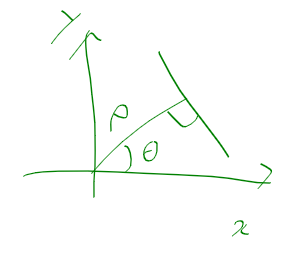
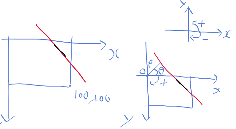
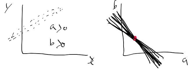
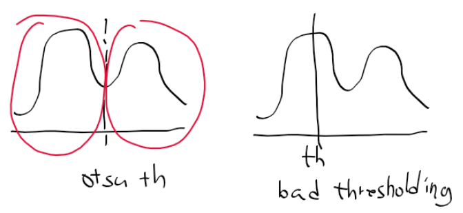
오늘 좌표계 때문에 손놓고 있던 허프 변환 문제를
겨우 겨우 해결해서 돌릴수가 있엇는데
내가 그동한 구현한 알고리즘들을
실제 사용하기에는 실행 속도가 너무 느렸다.
그러던 중에 이 알고리즘 설명, 구현 코드있던 사이트에서
픽셀 단위로 루프를 돌리는게 아닌
행렬 처리로 구하는 코드도 같이 구현해 두었더라.
그래서 한번 내가 보면서 구현한 코드랑
opencv 속도
벡터화 된 알고리즘 속도를 비교해보았다.
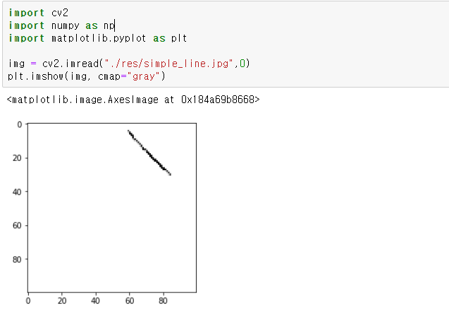
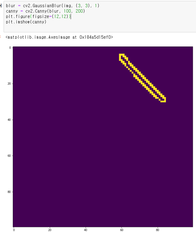
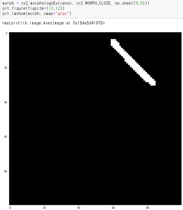
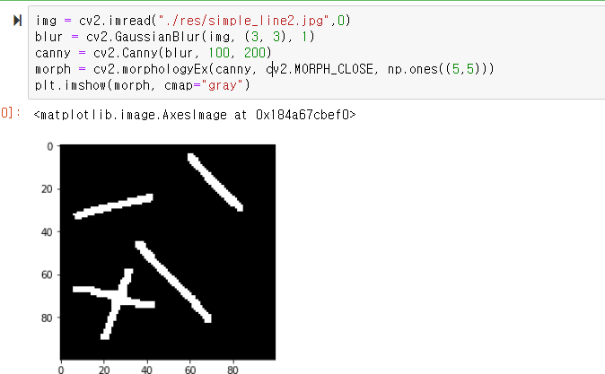
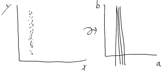
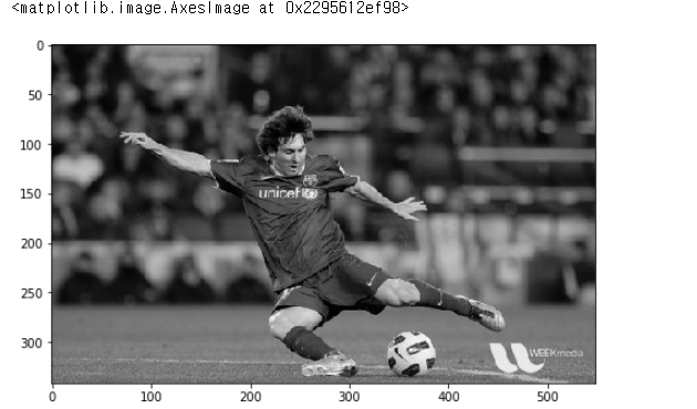
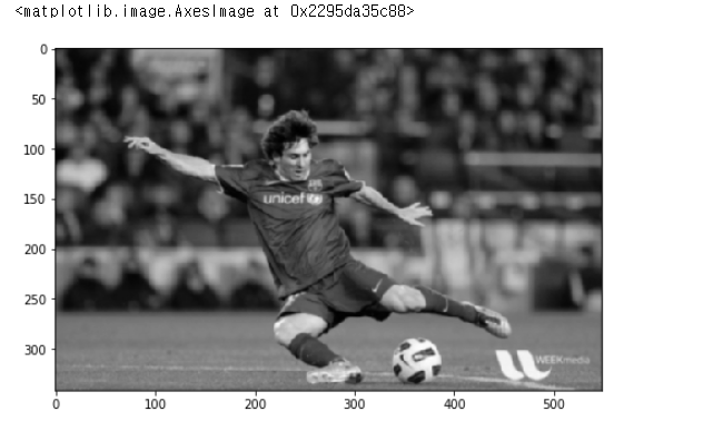
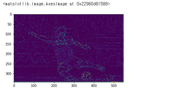
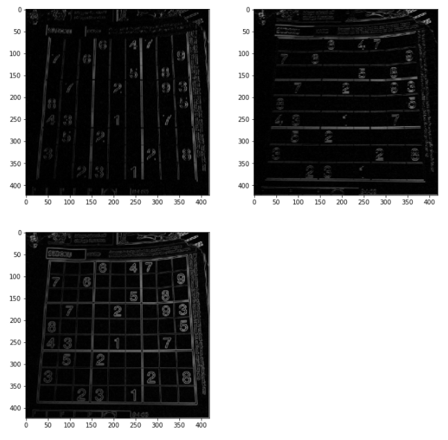
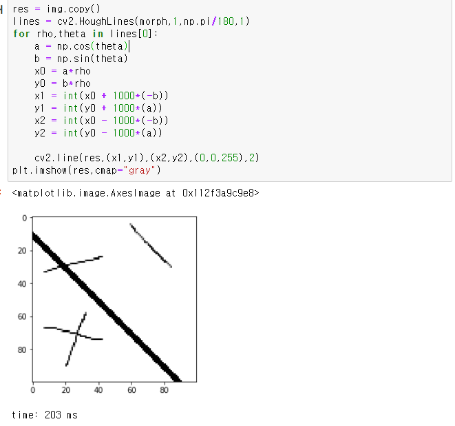
1. 픽셀 단위 처리를 통한 허프 라인 검출
에지 영상을 이미지로 주어 검출해보았는데
100 x 100 이미지임에도 2초 가까이 걸렷다.
opencv에선 어떨가
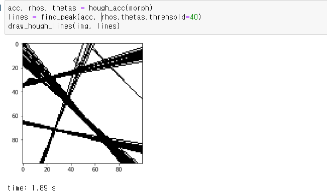
2. opencv houghline 함수 사용한 경우
위와 동일한 이미지에 opencv 함수만 사용해서 구해본 결과
200ms 정도 걸렸다.
위에서 구현한것보다 1/10 속도
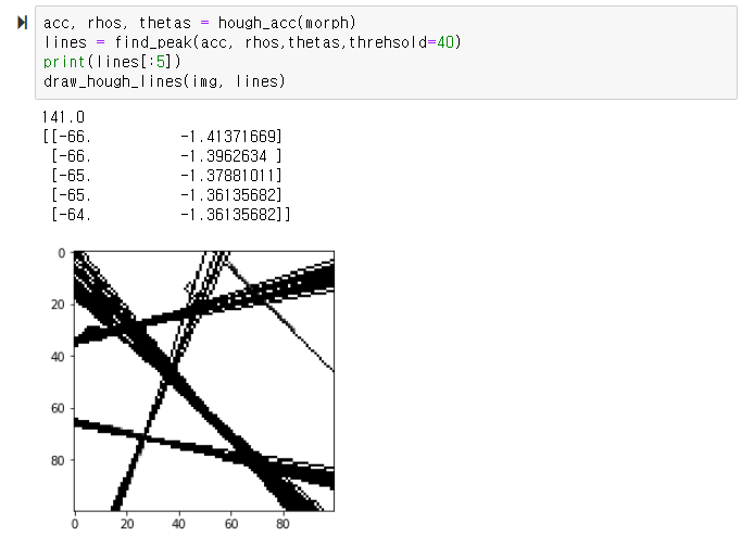
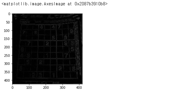
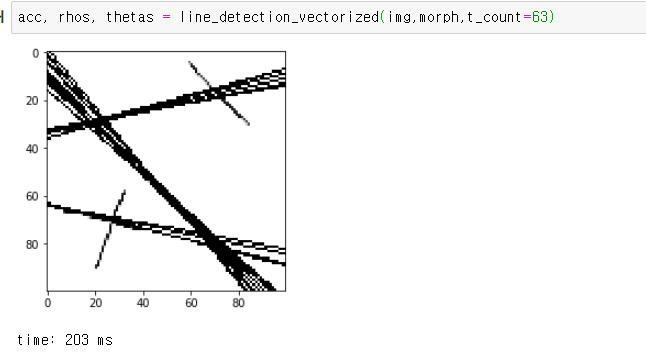
3. 행렬 처리를 통한 허프 라인 검출
ref : towardsdatascience.com/lines-detection-with-hough-transform-84020b3b1549
이 사이트에서 소개하는 코드를 필요 없는 부분을 빼고 돌릴수 있게 고쳤다.
고친 결과 opencv와 동일한 속도를 보이더라
위 시험을 위한 수정 코드
def line_detection_vectorized(image, edge_image, num_rhos=180, num_thetas=180, t_count=220):
    res = image.copy()
    edge_height, edge_width = edge_image.shape[:2]
    edge_height_half, edge_width_half = edge_height / 2, edge_width / 2

    d = np.sqrt(np.square(edge_height) + np.square(edge_width))
    dtheta = 180 / num_thetas
    drho = (2 * d) / num_rhos

    thetas = np.arange(0, 180, step=dtheta)
    rhos = np.arange(-d, d, step=drho)

    cos_thetas = np.cos(np.deg2rad(thetas))
    sin_thetas = np.sin(np.deg2rad(thetas))

    accumulator = np.zeros((len(rhos), len(rhos)))

    edge_points = np.argwhere(edge_image != 0)
    edge_points = edge_points - np.array([[edge_height_half, edge_width_half]])
    #
    rho_values = np.matmul(edge_points, np.array([sin_thetas, cos_thetas]))

    accumulator, theta_vals, rho_vals = np.histogram2d(
      np.tile(thetas, rho_values.shape[0]),
      rho_values.ravel(),
      bins=[thetas, rhos]
    )
    accumulator = np.transpose(accumulator)
    lines = np.argwhere(accumulator > t_count)

    for line in lines:
        y, x = line
        rho = rhos[y]
        theta = thetas[x]
        a = np.cos(np.deg2rad(theta))
        b = np.sin(np.deg2rad(theta))
        x0 = (a * rho) + edge_width_half
        y0 = (b * rho) + edge_height_half
        x1 = int(x0 + 1000 * (-b))
        y1 = int(y0 + 1000 * (a))
        x2 = int(x0 - 1000 * (-b))
        y2 = int(y0 - 1000 * (a))
        res = cv2.line(res, (x1, y1), (x2, y2), (0, 255, 0), 1)

    plt.imshow(res,cmap="gray")
    return accumulator, rhos, thetas
일단 이 문제를 행렬 연산으로 풀수 있으면
상당히 성능 개선할수 있는점을 볼수 있었다.
수정한 행렬 연산 코드를 나눠서 살펴보면
처음 대부분은 같은데
np.argwhere(edge_img != 0)을 사용한다.
np.argwhere(조건) 함수는 조건에 해당하는 인덱스를 반환해주더라
theta_resolution = 1
rho_resolution = 1
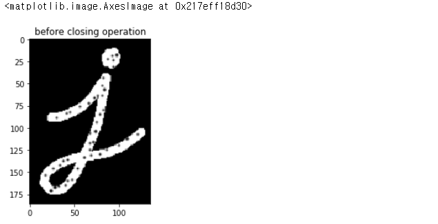
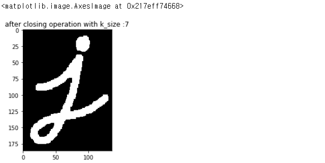
edge_img = morph.copy()
edge_height, edge_width = edge_img.shape
edge_height_half, edge_width_half = edge_height/2, edge_width/2
d = np.sqrt(np.square(edge_height) + np.square(edge_width))
thetas = np.arange(0, 180, theta_resolution)
rhos = np.arange(-d, d, rho_resolution)
cos_thetas = np.cos(np.deg2rad(thetas))
sin_thetas = np.sin(np.deg2rad(thetas))
accumulator = np.zeros((len(rhos), len(thetas)))
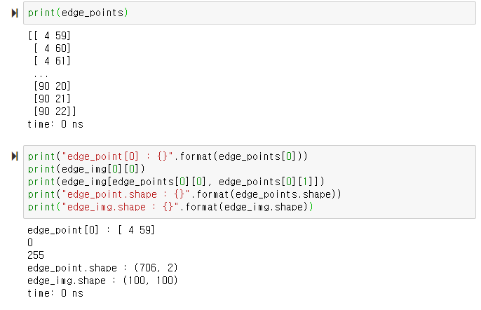
edge_points = np.argwhere(edge_img != 0)
edge_point는 조건에 맞는 인덱스 값들로 n x 2의 행렬 형태로 되어있다.
이미지가 100 x 100으로 1만 개의 픽셀이라면
edge_point는 706 x 2로 706개의 픽셀을 찾았다.
그다음에
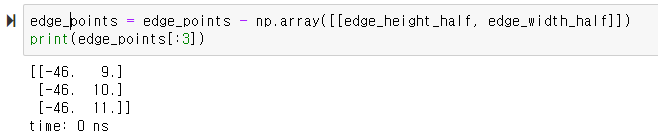
edge_points - 가로/2, 세로/2해주는데
이 연산으로
이미지를 중심점(h/2, w/2)을 중심으로 위치했던 요소들이
원점(0,0)을 중심으로 이동하게 된다.
그 다음
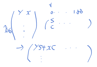
edge_point와 [sin_thetas, cos_thetas]의 행렬 곱 연산을 수행한다.
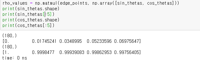
이 의미를 천천히 보면
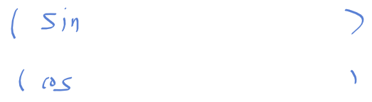
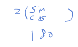
sin_thetas와 cos_thetas는 길이가 180인 벡터로
np.array()로 묶어주면
2 x 180의 행렬이 된다.
edge_points는
706 x 2형태의 행렬로 y, x 위치를 가지고 있으니
이 둘을 행렬 곱을 하면 706 x 180의 형태가 되며
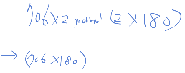
행렬 곱의 결과는
존재하는 모든 에지 포인트의 y, x와 모든 범위의 s, c를 곱 한 후 더한 것으로 rho가 나오게 된다.
정리하면 모든 경우의 rho를 구하게 된다.
행이 i 번째 에지 포인트
열은 j 번째 theta_index
이 행렬[i, j] = rho 값이 된다.
그 다음에는 히스토그램2d 함수로
누적결과와 theta_vals, rho_vals를 받고 있는데
우선 내부 내용들 부터 살펴보자
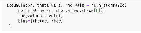
np.tile은 처음 보는 함수인대
np.tile(a, b)
- a 배열을 b만큼 복사를 해준다고 한다.
ref : numpy.org/doc/stable/reference/generated/numpy.tile.html
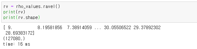
thetas는 180, rho_values 708 x 180이므로
np.tile로 구한 값은 708 x 180 = 127080이 된다.
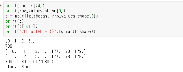
np.ravel()
- 주어진 배열을 1차원으로 평평 하게 만들어 준다.
ref : numpy.org/doc/stable/reference/generated/numpy.ravel.html
rho_values.ravel()로 모든 값들을 평활화 시켜주게 된다.
그다음 histogram2d를 보면
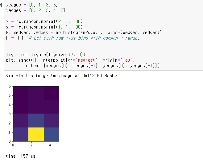
np.histogram2d
-numpy.histogram2d(x, y, bins=10, range=None, normed=None, weights=None, density=None)
- x : x vals
- y : y vals
- bins : binding vals
ref : numpy.org/doc/stable/reference/generated/numpy.histogram2d.html
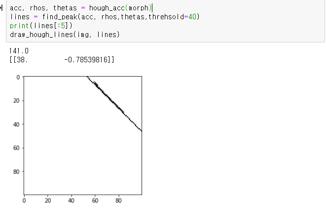
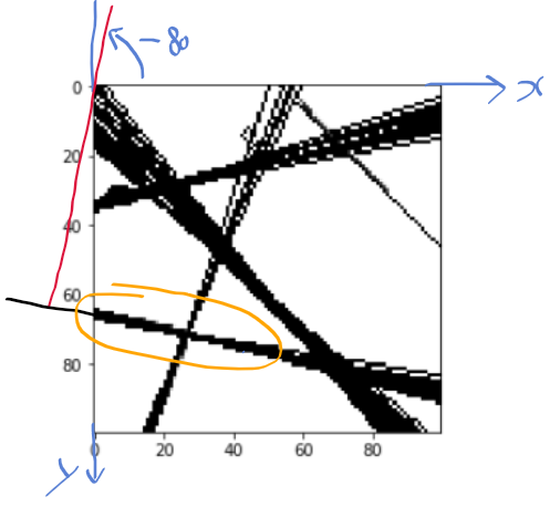
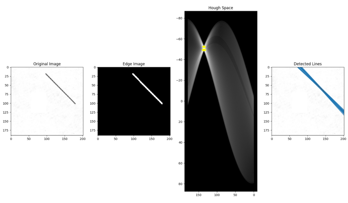
이제 누적기를 위한 np.histogram2d를 수행한 결과
허프 공간이 나오고
5개의 점이 가장 진하게 보인다.
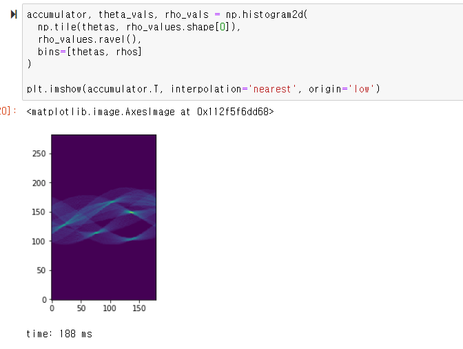
허프 공간을 구했으니
남은건 임계화와 시각화
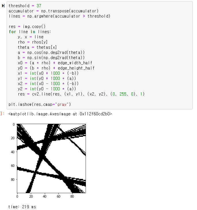
정리 - 행렬 연산을 통한 허프 라인 검출
def hough_line(edge_img, rho_resolution= 1, theta_resolution = 1, threshold=10):
    edge_height, edge_width = edge_img.shape
    edge_height_half, edge_width_half = edge_height/2, edge_width/2
    d = np.sqrt(np.square(edge_height) + np.square(edge_width))

    thetas = np.arange(0, 180, theta_resolution)
    rhos = np.arange(-d, d, rho_resolution)
    cos_thetas = np.cos(np.deg2rad(thetas))
    sin_thetas = np.sin(np.deg2rad(thetas))

    accumulator = np.zeros((len(rhos), len(thetas)))
    edge_points = np.argwhere(edge_img != 0)

    edge_points = edge_points - np.array([[edge_height_half, edge_width_half]])
    rho_values = np.matmul(edge_points, np.array([sin_thetas, cos_thetas]))

    accumulator, theta_vals, rho_vals = np.histogram2d(
      np.tile(thetas, rho_values.shape[0]),
      rho_values.ravel(),
      bins=[thetas, rhos]
    )
    accumulator = np.transpose(accumulator)
    lines = np.argwhere(accumulator > threshold)

    res = img.copy()
    for line in lines:
        y, x = line
        rho = rhos[y]
        theta = thetas[x]
        a = np.cos(np.deg2rad(theta))
        b = np.sin(np.deg2rad(theta))
        x0 = (a * rho) + edge_width_half
        y0 = (b * rho) + edge_height_half
        x1 = int(x0 + 1000 * (-b))
        y1 = int(y0 + 1000 * (a))
        x2 = int(x0 - 1000 * (-b))
        y2 = int(y0 - 1000 * (a))
        res = cv2.line(res, (x1, y1), (x2, y2), (0, 255, 0), 1)

    plt.imshow(res,cmap="gray")
    return accumulator, rhos, thetas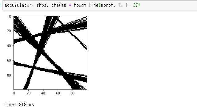
'로봇 > 영상' 카테고리의 다른 글
| 컴퓨터 비전 알고리즘 구현 - 12. 허프 변환을 이용한 직선 검출 구현 (0) | 2020.12.05 |
|---|---|
| 컴퓨터 비전 알고리즘 구현 - 11. 허프 변환 (0) | 2020.12.03 |
| 컴퓨터 비전 알고리즘 구현 - 10. 캐니 에지 검출기 만들기 (0) | 2020.12.01 |
| 컴퓨터 비전 알고리즘 구현 - 9. 이미지 그라디언트 (0) | 2020.11.30 |
| 컴퓨터 비전 알고리즘 구현 - 8. 모폴로지 연산 (0) | 2020.11.30 |