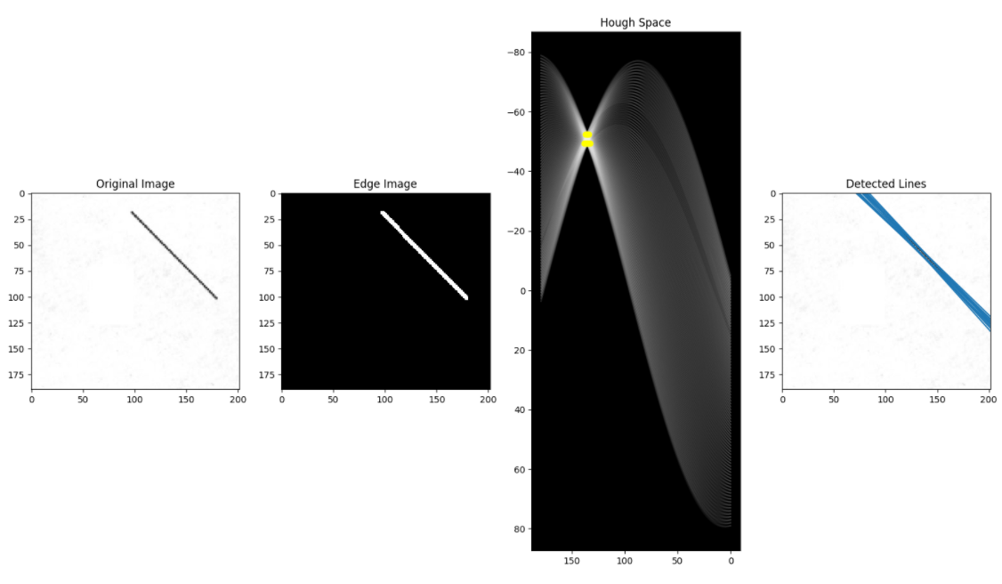
3. 에지 영상의 모든 픽셀 확인. 에지 픽셀에 대해서 가능한 모든 theta와 rho를 구하여 허프 행렬에 해당 인덱스 증감
4. 지정한 임계치를 넘는 값의 인덱스(rho, theta)가 검출된 직선
알고리즘 구현 자체는
여러 링크에 있는 내용들을 참고하다보니
대강 형태는 금방 만들었지만
시각화 할때가 많이 복잡했다.
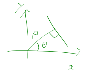
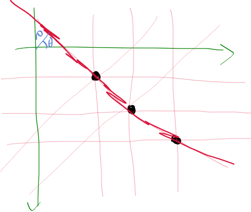
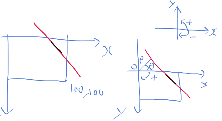
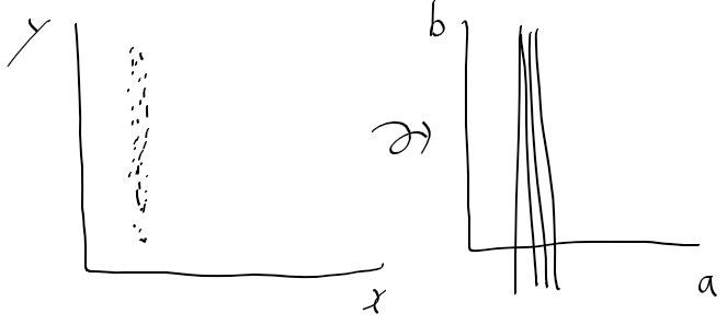
이전 글에서 일반적인 xy 좌표계 상에서 rho, theta를 놓으면 아래 그림과 같이 그릴수 있지만
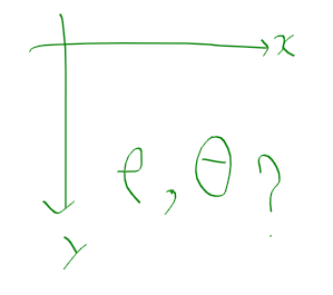
이미지 영역의 경우 y가 반대로 되어있는데
이때 rho, theta를 어떻게 보는 지가 문제였다.
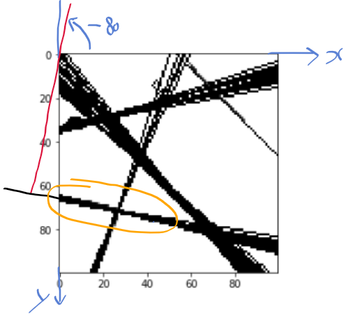
제대로 이해하지 않은 상태에서 하다보니
rho와 theta를 xy 좌표계상에서 라인 플로팅을 할때,
rho와 theta로 그린 라인이 내가 생각했던 대로가 아니거나, 실제 에지와 일치 하지 않게 계속 나오더라
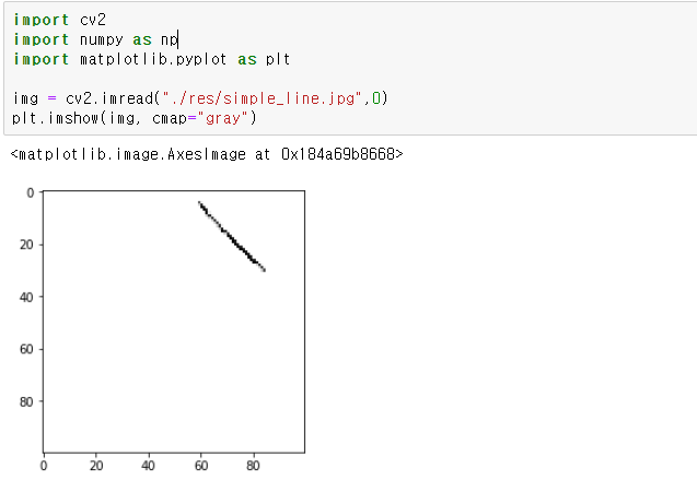
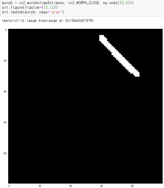
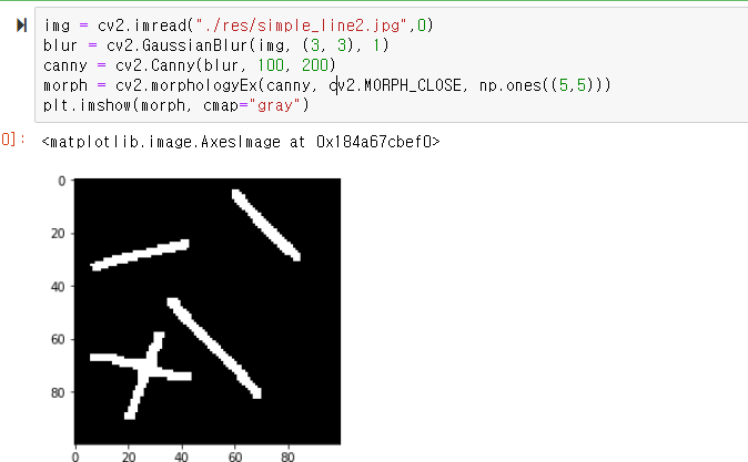
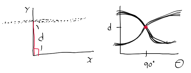
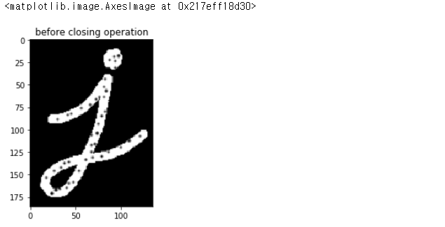
일단 사용한 기본 영상은 그림판에다가 일직선을 그려서 만들어봤다.
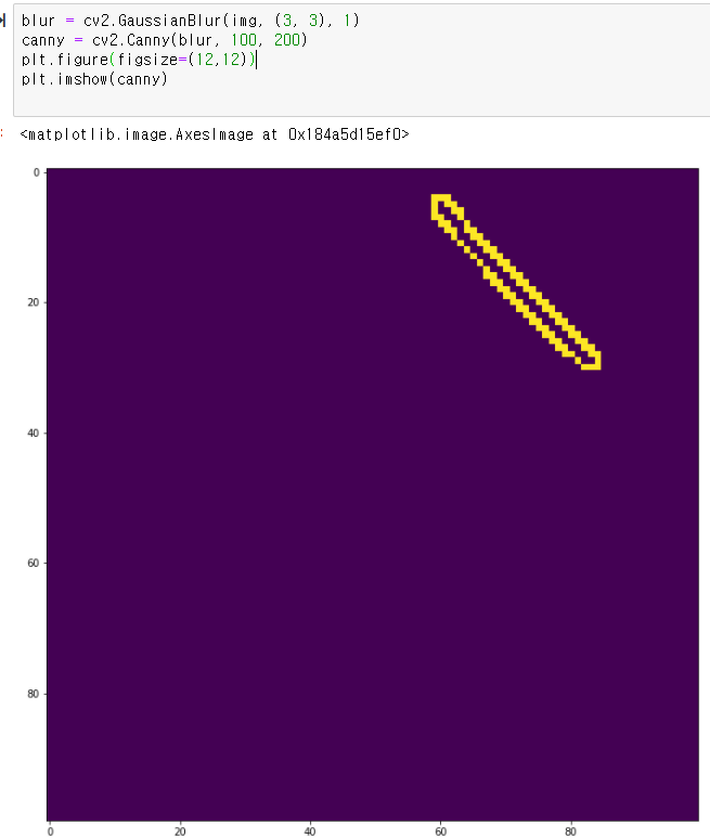
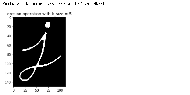
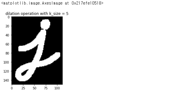
가우시안 블러링과 캐니 에지를 만들어주고
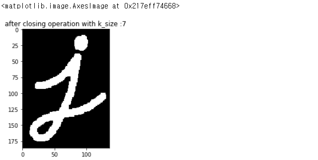
아무 생각없이(안해도 되지만) 모폴로지 닫힘도 해주었다.
이제 이 에지 영상에서 부터 시작하면 된다.
hough 공간의 누적 행렬을 만드는 함수를 구현하였다.
여기서 누적을 하는 이유는 많이 사용되는(임계치를 넘는) rho와 theta를 찾아 직선을 그려주기 위함인데,
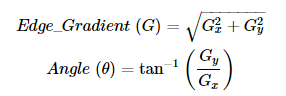
하나의 에지 픽셀에 대해서 모든 방향 360도 -> 직선으로 나타낼태니 180도를 1도 간격(해상도)으로 나누어
각 에지의 180도 rho를 구하고
해당 rho값 자체(rho)와 theta의 인덱스(theta_idx)를
누적 행렬의 행과 열 인덱스로 사용하고 1씩 증감을 시켰다.
accumulator[rho, theta_idx] += 1
def hough_acc(edge_img, rho_resolution= 1, theta_resolution = 1):
    rows, cols = edge_img.shape
    d = np.round(np.sqrt(rows**2 + cols**2))
    thetas = np.arange(-90, 90, theta_resolution)
    rhos = np.arange(-d, d + 1, rho_resolution)

    #all cos, sin thetas 0 from 180 degree
    cos_thetas = np.cos(np.deg2rad(thetas))
    sin_thetas = np.sin(np.deg2rad(thetas))
    accumulator = np.zeros((len(rhos), len(thetas)))
    cnt = 0
    for row in range(rows):
        for col in range(cols):
            # if seletecd point is edge
            if edge_img[row, col] != 0:
                cnt += 1
                # check all possible thetas
                for theta_idx in range(len(thetas)):
                    # rho = (x_dist * cos(theta)) + (y_dist * sin(theta))
                    rho =int(d + (col* cos_thetas[theta_idx])+(row *sin_thetas[theta_idx]))
                    accumulator[rho, theta_idx] += 1
    return accumulator, rhos, thetas
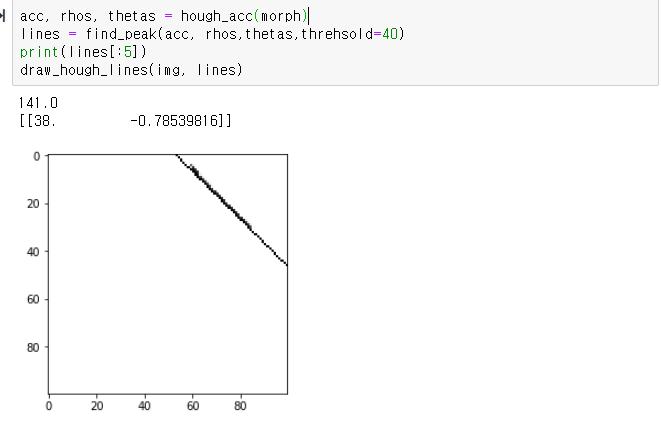
위 함수로부터 acc와 rhos, theta를 전달받아 임계치를 넘는
rho와 theta들을 모아 반환해주는 함수를 구현하였다.
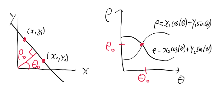
예를 들자면 아래와 같이 점 3개가 있는데
각 점에서 모든 방향으로 누적을 시키게 된다.
하지만 세점이 이어진 직선이 세 번 겹치므로 accumulator에서 가장 큰 값을 가지게 된다.
이 때, accumulator[rho, theta_idx] = 겹친 횟수이며
이 겹친 횟수가 임계치를 넘으면 직선으로 포함시킨다.
def find_peak(accumulator, rhos, thetas, threhsold=60):

    lines = []
    for y in range(accumulator.shape[0]):
        rho = rhos[y]
        for x in range(accumulator.shape[1]):
            if accumulator[y][x] > threhsold:
                theta = np.deg2rad(thetas[x])
                lines.append([rho, theta])

    return np.array(lines)
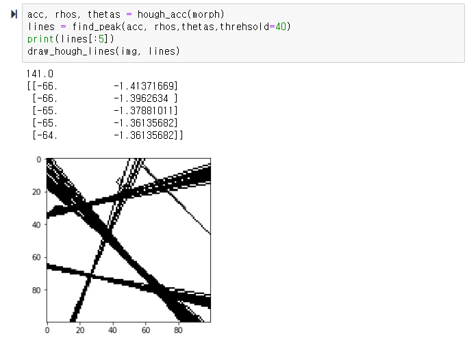
마지막으로 원본 이미지와
위 함수에서 반환한 직선으로
라인을 플로팅 시키는 함수
rho와 theta로 부터
직선을 구하는데
x0, y0가 (그리고자 하는) 법선과 만나는 점이고,
x1,y1 x2,y2는 이미지 밖에서 부터 그려주기 위해 구한 좌표가 된다.
def draw_hough_lines(img, lines):
    res = img.copy()
    for i, line in enumerate(lines):
        rho = line[0]
        theta = line[1]
        # reverse engineer lines from rhos and thetas
        a = np.cos(theta)
        b = np.sin(theta)
        x0 = a*rho
        y0 = b*rho

        # these are then scaled so that the lines go off the edges of the image
        x1 = int(x0 + 1000*(-b))
        y1 = int(y0 + 1000*(a))
        x2 = int(x0 - 1000*(-b))
        y2 = int(y0 - 1000*(a))
        cv2.circle(res, (int(x0), int(y0)),2,(0,0,255),1)
        cv2.line(res, (x1, y1), (x2, y2), (0, 255, 0), 1)
        plt.imshow(res,cmap="gray")
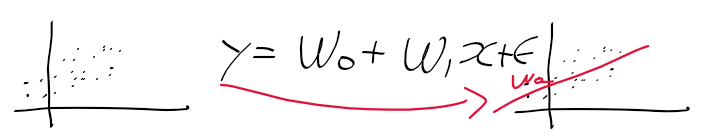
- 입력 벡터(독립 변수) x와 계수 벡터(가중치 벡터) w의 선형 결합으로 종속 변수 y를 예측하는 모델
- x = [0, x1, x2, x3 ..., x_p]
- w = [w0, w1, w2, ..., x_p]
- y = w.dot(x) = w0 + w1 x1 + . . . + w_p x_p
Linear Regression
- MSE를 최소화 하는 계수 벡터로 구한 선형 회귀 모델
- 독립 변수 간의 상관 관계가 높을 수록 분산, 오류가 커짐 : 다중 공선성 multi collinearity 문제
=> 독립적이고, 중요한 변수, 피처 위주로 남기거나 규제 or PCA 수행
회귀 모델 평가 지표
- MAE Mean Absolute Error : sum(|y - y_hat|) -> 일반 오차 합
- MSE Mean Sqaured Error : sum( (y - y_hat)^2 ) -> 오차가 클수록 크게 반영됨
- RMSE Root Mean Squared Error : root(MSE) -> MSE가 과하게 커지는것을 방지
- R2 : var(y_hat) / var(y) = 예측 분산/ 실제 분산 -> 1에 가까울수록 잘 예측
회귀 모델에서 평가 지표 사용시 유의할 점
- 회귀 평가 지표들은 분류 평가 지표들과는 달리 오차의 합이므로 값이 작을 수록 오차가 작아 더 좋은 모델임
-> -1하여 음수로 만듬
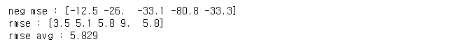
- 회귀 모델 스코어링 사용 시 "neg_mean_squared_error"와 같이 앞에 "neg_"를 붙여서 명시 해야 함.
1. 라이브러리 임포트
import numpy as np
import matplotlib.pyplot as plt
import seaborn as sns
import pandas as pd
from scipy import stats
from sklearn.datasets import load_boston
2. 데이터 로드
boston = load_boston()
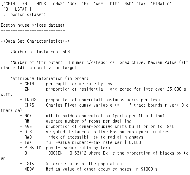
print(boston.feature_names)
print(boston.DESCR)
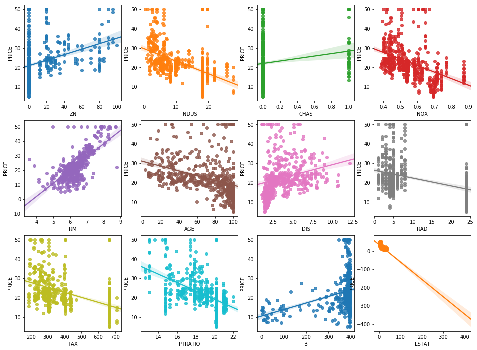
# ZN ~ LSTAT까지 각 변수들과 PRICE의 선형 관계를 sns.regplot으로 살펴보자
fix, axs = plt.subplots(figsize=(16, 12), ncols=4, nrows=3)
features = df.columns[1:-1]

for i, feature in enumerate(features):
    row = int(i/4)
    col = i%4
    sns.regplot(x=feature, y="PRICE", data=df, ax=axs[row][col])
6. 학습 및 평가 지표 살펴보기
from sklearn.model_selection import train_test_split
from sklearn.linear_model import LinearRegression
from sklearn.metrics import mean_squared_error, r2_score
y = df["PRICE"]
X = df.iloc[:,:-1]
X_train, X_test, y_train, y_test = train_test_split(X,y, test_size=0.2)
lr = LinearRegression()
lr.fit(X_train, y_train)
y_pred = lr.predict(X_test)
mse = mean_squared_error(y_test, y_pred)
r2 = r2_score(y_test, y_pred)
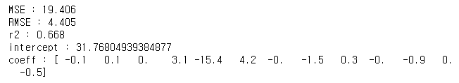
print("MSE : {0:.3f}".format(mse))
print("RMSE : {0:.3f}".format(np.sqrt(mse)))
print("r2 : {0:.3f}".format(r2))
print("intercept : {}".format(lr.intercept_))
print("coeff : {}".format(np.round(lr.coef_,1)))
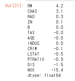
7. 피처 별 회귀 계수 살펴보기
- lr.coef_를 시리즈로 만들어 정렬 후 출력
- sns.regplot에서 본대로 RM은 강한 양의 상관 관계, LSTAT은 음의 상관관계를 가짐
- 독립 변수들과 하나의 종속 변수가 주어지고, 이에 대한 데이터들이 있을때 종속 변수를 가장 잘 추정하는 직선을 구하는 문제
- 새로운 데이터가 주어지면 학습 과정에서 구한 회귀선으로 연속적인 값을 추정할 수 있음.
- 선형 회귀 모델은 계수 벡터 beta = [beta0, . . ., beta_p], 독립 변수 벡터 x = [0, x1, ...., x_p]의 선형 결합의 형태가 됨.
- e는 오차 모형으로 기본적으로 평균 0, 분산이 1인 정규 분포를 따르고 있음.
-> 회귀 선과 추정한 y 사이의 오차를 의미함.
- 실제 종속 변수를 y, 주어진 독립변수를 통해 예측한(추정한) y를 y hat로 표기
- 오차 e는 y - y_hat으로 아래와 같은 관계를 가지고 있음.
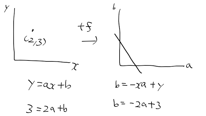
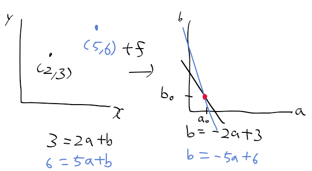
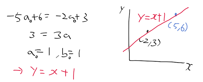
단순 선형 회귀 모형
- 독립 변수가 1개인 선형 회귀 모형
- 아래의 좌측과 같이 2차원 공간 상에 점들이 주어질때, 우측과 같은 선형 회귀 모델을 구할 수 있음
- 기존의 회귀 계수 beta를 여기선 가중치의 의미로 w로 표기함.
- 오차 = 실제 값 - 추정 값의 관계를 가짐.
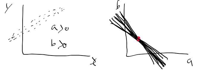
최소 제곱 오차 MSE : Mean Sqaured Error
- 실제 결과(y_i) - 추정 결과(y_i hat)의 제곱한 것을 모든 데이터에 대해 합한 후 데이터 갯수(N) 만큼 나누어 구한 오차
- 위의 산점도 데이터가 주어질떄 MSE를 최소가 되게하는 회귀 계수들로 선형 회귀 모델을 만듬
회귀 계수 구하기 기초
- MSE를 최소로 만드는 회귀 계수는 편미분을 통해 구할 수 있음.
- y = x^2라는 그래프가 주어질때, argmin(y)를 구하는 x를 얻으려면, y를 x로 편미분하여 0이 나오게하는 x를 구하면됨.
- d/dx y = 2x = 0 => x = 0일때 기울기는 0으로 y는 최소 값을 가짐
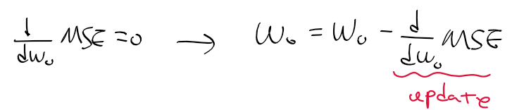
- 단순 선형 회귀 모델의 회귀 계수 구하는 방법 : MSE를 w0, w1에 편미분 한 후 0이 되도록 하는 w0, w1를 구함.
회귀 계수 구하기
- MSE를 w0, w1로 편미분하여 0이되는 w0, w1을 구하자
- n제곱 다항식의 미분에 대한 공식을 이용하여 w0, w1에 대해 편미분을 하면 아래와 같이 정리할 수 있음.
w0 회귀 계수 구하기
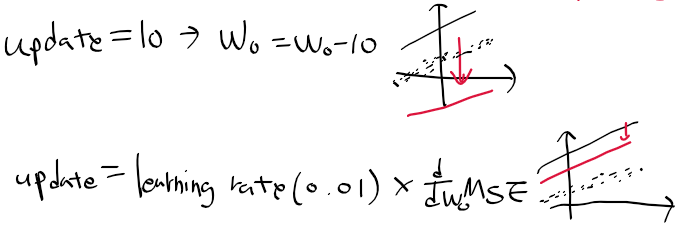
- 회귀 계수는 초기에 특정 값(주로 1)로 초기화 후 오차의 크기에 따라 갱신 값을 빼 조금씩 조정됨
- MSE를 w0로 편미분(갱신 값)하여 0이 되게 만드는 w0는 아래와 같이 구할 수 있음.
=> 기존의 회귀 계수(w0) - 기존 회귀 계수의 오차(갱신 값, d MSE/ d w0) = 새 회귀 계수(w0)
- 갱신 값이 너무 큰 경우, 올바른 회귀 모델을 구하기 힘들어짐
-> 학습률 learning rate를 통해 조금씩 오차를 조정해 나감.
2차원 데이터로 부터 단순 선형 회귀 모델 구하기
1. 데이터 준비
import numpy as np
import matplotlib.pyplot as plt

# y = w0 + w1 * x 단순 선형 회귀 식
# y = 4x + 6(w0 = 6, w1= 4)에 대한 선형 근사를 위해 값 준비
x = 2 * np.random.rand(100, 1) # 0 ~ 2까지 100개 임의의 점
y = 6 + 4 * x + np.random.randn(100, 1) # 4x + 6 + 정규 분포를 따르는 노이즈

plt.scatter(x, y)
2. 주어진 데이터에 적합한 회귀 모델 구하기
- 가중치(회귀 계수) 1로 초기화 -> 가중치 갱신 과정 수행(get_weight_update)
- x에 대한 추정한 y를 구함 -> 실제 y - 추정 y로 오차 diff 구함.
- 위에서 구한 가중치 갱신 공식에 따라 w0, w1의 갱신 값을 구함(w0/w1_update)
- 가중치 - 가중치 갱신 값. 이 연산을 지정한 횟수 만큼 수행
=> 회귀 계수는 일정한 값으로 수렴함 : 선형 회귀 모델의 회귀 계수.
def get_weight_update(w1, w0, x, y, learning_rate=0.01):
    # y는 길이가 100인 벡터, 길이 가져옴
    N = len(y)

    # 계수 w0, w1 갱신 값을 계수 w0, w1 동일한 형태로 초기화
    w1_update = np.zeros_like(w1)
    w0_update = np.zeros_like(w0)

    # 주어진 선형 회귀 식을 통한 값 추정
    y_pred = np.dot(x, w1.T) + w0
    # 잔차 y - hat_y
    diff = y - y_pred

    # (100, 1) 형태의 [[1, 1, ..., 1]] 행렬 생성, diff와 내적을 구하기 위함.
    w0_factors = np.ones((N, 1))

    # 우측의 식은 MSE를 w1과 w0에 대해 편미분을 하여 구함.
    # d mse/d w0 = 0 이 되게하는 w0이 mse의 최소로 함
    # d mse/d w1 = 0 이 되게하는 w1이 mse를 최소로 함
    # 급격한 w0, w1 변화를 방지 하기 위해 학습률 learning_rate 사용

    w1_update = -(2/N) * learning_rate * (np.dot(x.T, diff))
    w0_update = -(2/N) * learning_rate * (np.dot(w0_factors.T, diff))

    return w1_update, w0_update

def gradient_descent_steps(X, y, iters= 10000):

    w0 = np.zeros((1, 1))
    w1 = np.zeros((1, 1))

    for idx in range(0, iters):

        w1_update, w0_update = get_weight_update(w1, w0, X, y, learning_rate=0.01)
        # 갱신 값으로 기존의 w1, w0을 조정해 나감
        w1 = w1 - w1_update
        w0 = w0 - w0_update

    return w1, w0

def get_cost(y, y_pred):
    N = len(y)
    cost = np.sum(np.square(y- y_pred))/N
    return cost

w1, w0 = gradient_descent_steps(x, y, iters=1000)
print("w1:{0:.4f}, w0:{0:.4f}".format(w1[0, 0], w0[0, 0]))
y_pred = w1[0, 0] * x + w0
print("gradient descent total cost : {0:.4f}".format(get_cost(y, y_pred)))
"""
Canny Edge Detector
- 2020. 12.1 01:50
"""
"""
ref
- https://en.wikipedia.org/wiki/Canny_edge_detector
"""
def sobel_kerenl():
kernel_x = np.array([
[-1, 0, 1],
[-2, 0, 2],
[-1, 0, 1]
])
kernel_y = np.array([
[1, 2, 1],
[0, 0, 0],
[-1, -2, -1]
])
return kernel_x, kernel_y
def get_rounded_gradient_angle(ang):
"""
get_rounded_gradient_angle
- gradient direction angle round to one of four angles
return : one of four angles
representing vertical, horizontal and two diagonal direction
parameteres
---------------
ang : gradient direction angle
"""
vals = [0, np.pi*1/4, np.pi*2/4, np.pi*3/4, np.pi*4/4]
interval = [np.pi*1/8, np.pi*3/8, np.pi * 5/8, np.pi* 7/8]
if ang < interval[0] and ang >= interval[-1]:
ang = vals[0]
elif ang < interval[1] and ang >= interval[0]:
ang = vals[1]
elif ang < interval[2] and ang >= interval[1]:
ang = vals[2]
elif ang < interval[3] and ang >= interval[2]:
ang = vals[3]
else:
ang = vals[4]
return ang
def get_gradient_intensity(img):
"""
get gradient_intensity
- calculate gradient direction and magnitude
return (rows, cols, 2) shape of image about grad direction and mag
parameteres
------------
img : blured image
"""
k_size = 3
rows, cols = img.shape
kernel_x, kernel_y = sobel_kerenl()
pad_img = padding(img, k_size=k_size)
res = np.zeros((rows, cols, 2))
sx, sy = 0, 0
for i in range(0, rows):
for j in range(0, cols):
boundary = pad_img[i:i+k_size, j:j+k_size]
sx = np.sum(kernel_x * boundary)
sy = np.sum(kernel_y * boundary)
ang = np.arctan2(sy, sx)
mag = abs(sx) + abs(sy)
if ang < 0:
ang = ang + np.pi
ang = get_rounded_gradient_angle(ang)
res[i, j, 0] = ang
res[i, j, 1] = mag
return res
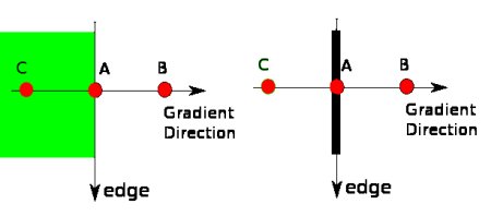
def check_local_maximum(direction=None, boundary=None):
"""
check_local_maximum
- check if center value is local maximum depend on gradient direction
return True if center valus is local maximum
parameter
------------
direction : gradient direction
boundary : region of image for finding local maximum
"""
if direction == 0: # 0 degree, east and west direction
kernel = np.array([
[0, 0, 0],
[1, 1, 1],
[0, 0, 0]
])
elif direction == 1: #45 degree, north east and south west direction
kernel = np.array([
[0, 0, 1],
[0, 1, 0],
[1, 0, 0]
])
elif direction == 2: #90 degree, north & south direction
kernel = np.array([
[0, 1, 0],
[0, 1, 0],
[0, 1, 0]
])
else : #135 degree, north west & south east direction
kernel = np.array([
[1, 0, 0],
[0, 1, 0],
[0, 0, 1]
])
max_val = np.max(kernel * boundary)
if boundary[1,1] == max_val: #local maximum
return True
else: # not local maximu
return False
def non_maximum_suppression(grad_intensity=grad_intensity):
"""
non_maximum_suppression
- check a pixel wiht it's neighbors in the direction of gradient
- if a pixel is not local maximum, it is suppressed(means to be zero)
"""
directions = [0, np.pi*1/4, np.pi*2/4, np.pi*3/4, np.pi*4/4]
k_size = 3
grad_direction = grad_intensity[:, :, 0]
grad_magnitude = grad_intensity[:, :, 1]
rows, cols = grad_magnitude.shape
pad_img = padding(grad_magnitude, k_size=k_size)
res_img = np.zeros((rows,cols))
sx, sy = 0, 0
for i in range(0, rows):
for j in range(0, cols):
direction = directions.index(grad_direction[i,j])
boundary = pad_img[i:i+k_size, j:j+k_size]
if check_local_maximum(direction, boundary) == True:
res_img[i, j] = grad_magnitude[i, j]
else:
res_img[i, j] = 0
return res_img
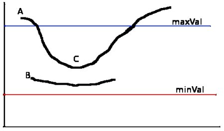
def hysteresis_threshold(suppressed_img=None, min_th=None, max_th=None):
"""
hysterisis_threshold
- check edge is connected to strong edge using eight connectivity
parameter
---------------------
- suppressed img : non maximum suppressed image
- min_th : minimal threshold value
- max_th : maximum threshold value
"""
k_size = 3
rows, cols = supressed_img.shape
pad_img = padding(suppressed_img, k_size=k_size)
res_img = np.zeros((rows,cols))
eight_connectivity = np.array([
[1, 1, 1],
[1, 0, 1],
[1, 1, 1]
])
for i in range(0, rows):
for j in range(0, cols):
if pad_img[i+1, j+1] < min_th:
res_img[i, j] = 0
else:
boundary = pad_img[i:i+k_size, j:j+k_size]
max_magnitude = np.max(boundary * eight_connectivity)
if max_magnitude >= max_th : # pixel is connected to real edge
res_img[i, j] = 255
else:
res_img[i, j] = 0
return res_img
def canny_edge_detector(img=None, min_th=None, max_th=None):
"""
canny_edge_detector
- detect canny edge from original image
parameter
- img : original image
- min_th : minimal threshold value
- max_th : maximum threshold value
"""
img_blur = gaussian_filtering(img,k_size=5, sigma=1)
grad_intensity = get_gradient_intensity(img_blur)
suppressed_img = non_maximum_suppression(grad_intensity)
canny_edge = hysteresis_threshold(suppressed_img=suppressed_img,
min_th=min_th, max_th=max_th)
return canny_edge
def canny_edge_visualize(img, min_th=100, max_th=200):
"""
canny_edge_visualize
- visualize all images from original to canny edge
parameter
- min_th : minimal threshold value
- max_th : maximum threshold value
"""
img_blur = gaussian_filtering(img,k_size=5, sigma=1)
grad_intensity = get_gradient_intensity(img_blur)
suppressed_img = non_maximum_suppression(grad_intensity)
canny_edge = hysteresis_threshold(suppressed_img=suppressed_img,min_th=100, max_th=200)
plt.figure(figsize=(64,32))
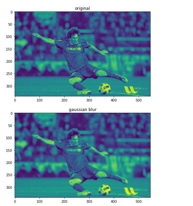
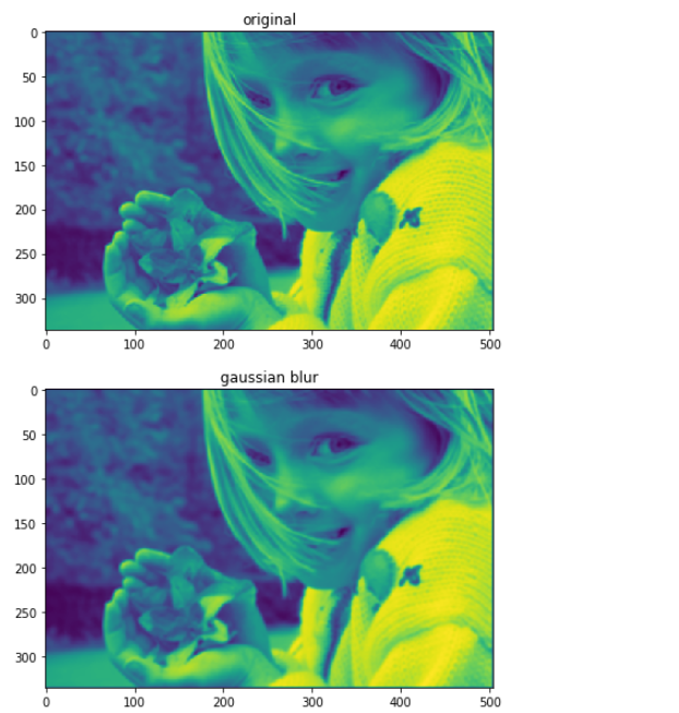
plt.subplot(6, 1, 1)
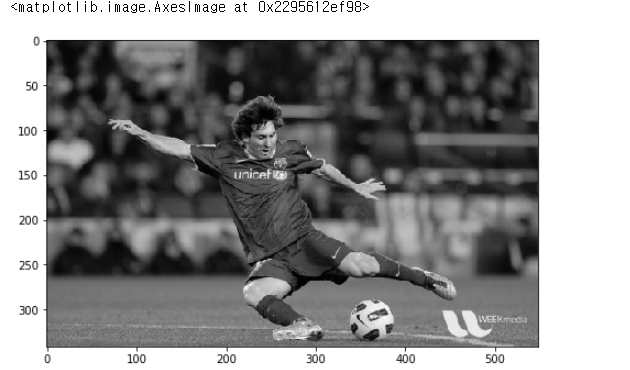
plt.title("original")
plt.imshow(img)
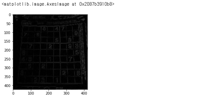
plt.subplot(6, 1, 2)
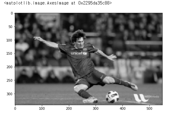
plt.title("gaussian blur")
plt.imshow(img_blur)
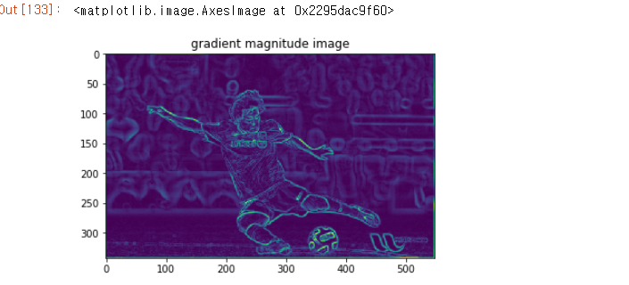
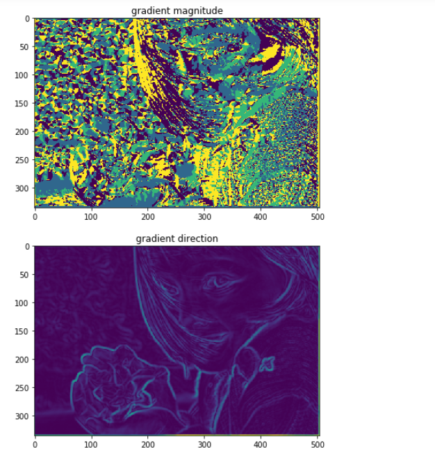
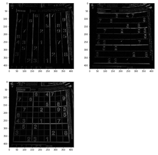
plt.subplot(6, 1, 3)
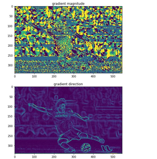
plt.title("gradient magnitude")
plt.imshow(grad_intensity[:, :,0])
plt.subplot(6, 1, 4)
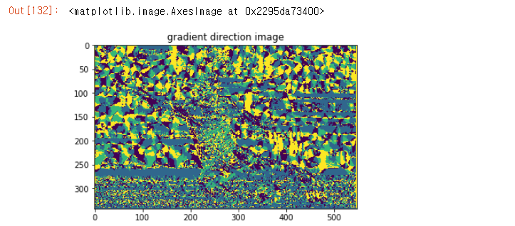
plt.title("gradient direction")
plt.imshow(grad_intensity[:, :,1])
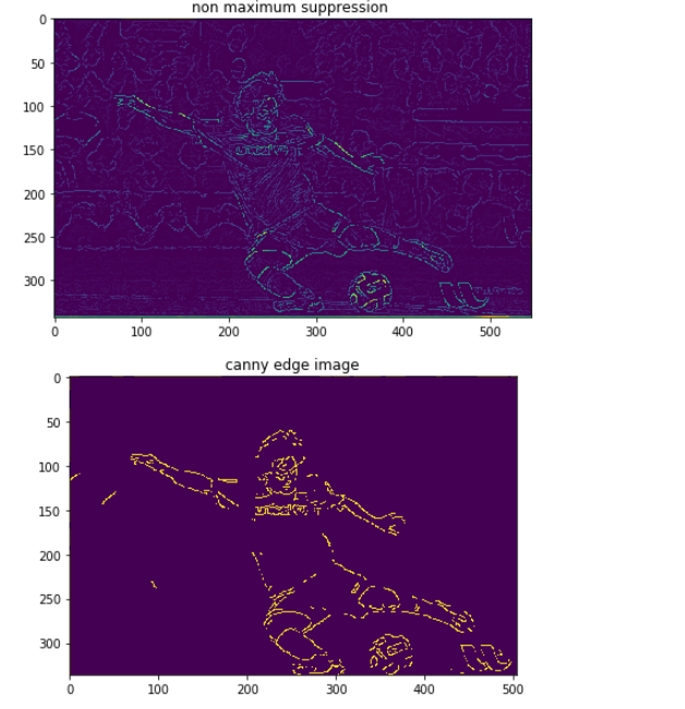
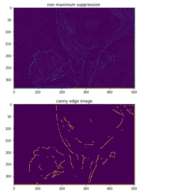
plt.subplot(6, 1, 5)
plt.title("non maximum suppression ")
plt.imshow(suppressed_img)
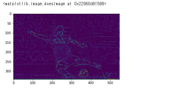
plt.subplot(6, 1, 6)
plt.title("canny edge image")
plt.imshow(canny_edge)
- 기본 모델로 knn, random forest, adaboost, decisiont tree 4가지
- 마지막 모델로 logistic regression
import numpy as np
from sklearn.neighbors import KNeighborsClassifier
from sklearn.ensemble import RandomForestClassifier
from sklearn.ensemble import AdaBoostClassifier
from sklearn.tree import DecisionTreeClassifier
from sklearn.linear_model import LogisticRegression

from sklearn.datasets import load_breast_cancer
from sklearn.model_selection import train_test_split
from sklearn.metrics import accuracy_score
from utils.common import show_metrics
2. 데이터 로드 및 조회
- 행 569, 열 30개 데이터
- 악성과 양성사이 큰 비율 차이는 없음
data = load_breast_cancer()
X = data.data
y = data.target
print(data.DESCR)

import pandas as pd
print(pd.Series(y).value_counts())
3. 각 분류기 학습, 성능 확인
- 각 분류기 학습 및 성능 출력, 예측 데이터 쌓기
- lr_final에 학습 용 데이터를 만들기 위해 예측 데이터 shape가 (4, 114) 인것을 전치. 114행 4열 데이터로 변환
The datasets contains transactions made by credit cards in September 2013 by european cardholders. This dataset presents transactions that occurred in two days, where we have 492 frauds out of 284,807 transactions. The dataset is highly unbalanced, the positive class (frauds) account for 0.172% of all transactions.
언더 샘플링, 오버샘플링
- 불균형 레이블 분포를 적절한 학습데이터로 만드는 방법, 오버 샘플링이 유리
- 언더 샘플링 : 클래스가 많은 데이터를 클래스가 적은 데이터 만큼 축소
ex. 정상 10,000건, 비정상 100건시 정상을 100건으로 줄임. *너무 많은 정상 데이터를 제거
- 오버 샘플링 : 클래스가 적은 데이터를 클래스가 많은 데이터 만큼 증가
* 단순 증강 시 오버피팅이 발생. 원본 데이터 피처를 약간씩 변형하여 증감
ex. SMOTE(Syntheic Minority Over sampling techinuqe : knn으로 적은 클래스 데이터 간의 차이로 새 데이터 생성
* imbalanced-learning 사용
1. 데이터로드
import numpy as np
import pandas as pd
import seaborn as sns
import matplotlib.pyplot as plt
import warnings
warnings.filterwarnings("ignore")

path = "./res/credit card fraud detection/creditcard.csv"
df = pd.read_csv(path)
df.head()
2. 전처리 및 훈련, 테스트 데이터 셋 분리 정의
from sklearn.model_selection import train_test_split

def get_preprocessed_df(df=None):
    """
    input
    df : before preprocessing

    output
    res : after dropping time columns
    """
    res = df.copy()
    res.drop("Time", axis=1, inplace=True)
    return res

def get_train_test_datasets(df=None):
    df_copy = get_preprocessed_df(df)
    X_features = df_copy.iloc[:,:-1]
    y_target= df_copy.iloc[:,-1]

    X_train, X_test, y_train, y_test = train_test_split(X_features, y_target,
                                                       test_size=0.2,
                                                       stratify=y_target,
                                                       random_state=100)
    return X_train, X_test, y_train, y_test
3. 로지스틱 회귀 모델로 성능 확인
- 정확도는 좋으나 재현률과 F1 스코어가 크게 떨어짐
X_train, X_test, y_train, y_test = get_train_test_datasets(df)

from sklearn.linear_model import LogisticRegression
from utils.common import show_metrics


lr = LogisticRegression()
lr.fit(X_train, y_train)
y_pred = lr.predict(X_test)
show_metrics(y_test, y_pred)