선형 회귀 모델 Linear Regression Model
- 입력 벡터(독립 변수) x와 계수 벡터(가중치 벡터) w의 선형 결합으로 종속 변수 y를 예측하는 모델
- x = [0, x1, x2, x3 ..., x_p]
- w = [w0, w1, w2, ..., x_p]
- y = w.dot(x) = w0 + w1 x1 + . . . + w_p x_p
Linear Regression
- MSE를 최소화 하는 계수 벡터로 구한 선형 회귀 모델
- 독립 변수 간의 상관 관계가 높을 수록 분산, 오류가 커짐 : 다중 공선성 multi collinearity 문제
=> 독립적이고, 중요한 변수, 피처 위주로 남기거나 규제 or PCA 수행
회귀 모델 평가 지표
- MAE Mean Absolute Error : sum(|y - y_hat|) -> 일반 오차 합
- MSE Mean Sqaured Error : sum( (y - y_hat)^2 ) -> 오차가 클수록 크게 반영됨
- RMSE Root Mean Squared Error : root(MSE) -> MSE가 과하게 커지는것을 방지
- R2 : var(y_hat) / var(y) = 예측 분산/ 실제 분산 -> 1에 가까울수록 잘 예측
회귀 모델에서 평가 지표 사용시 유의할 점
- 회귀 평가 지표들은 분류 평가 지표들과는 달리 오차의 합이므로 값이 작을 수록 오차가 작아 더 좋은 모델임
-> -1하여 음수로 만듬
- 회귀 모델 스코어링 사용 시 "neg_mean_squared_error"와 같이 앞에 "neg_"를 붙여서 명시 해야 함.
1. 라이브러리 임포트
import numpy as np
import matplotlib.pyplot as plt
import seaborn as sns
import pandas as pd
from scipy import stats
from sklearn.datasets import load_boston
2. 데이터 로드
boston = load_boston()
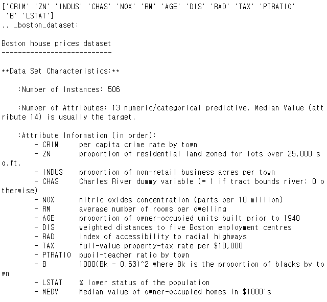
print(boston.feature_names)
print(boston.DESCR)
3. 데이터 프레임 변환, 훑어보기
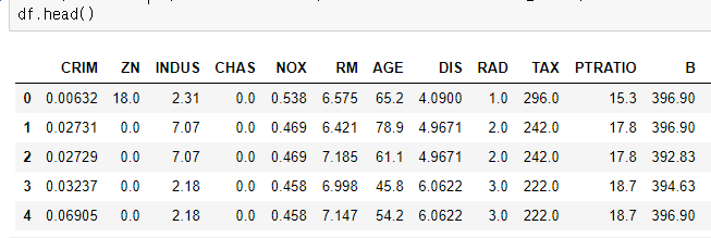
df = pd.DataFrame(data=boston.data, columns=boston.feature_names)
df.head()
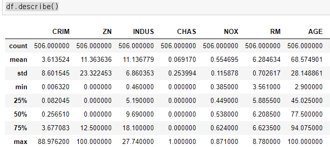
df.describe()
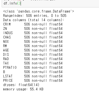
df["PRICE"] = boston.target
df.info()
4. 변수간 상관관계 보기
- sns.pairplot
- pairplot은 너무 오래 걸림
-> 각 독립변수와 종속변수의 상관관계를 보자

5. 각 독립변수와 종속변수 PRICE 사이 상관관계 보기
- sns.regplot() : 산점도와 회귀 선을 그려줌.
- 직선을 보면 RM은 PRICE와 강한 양의 상관관계
- LSAT은 PRICE와 강한 음의 상관관계를 가짐
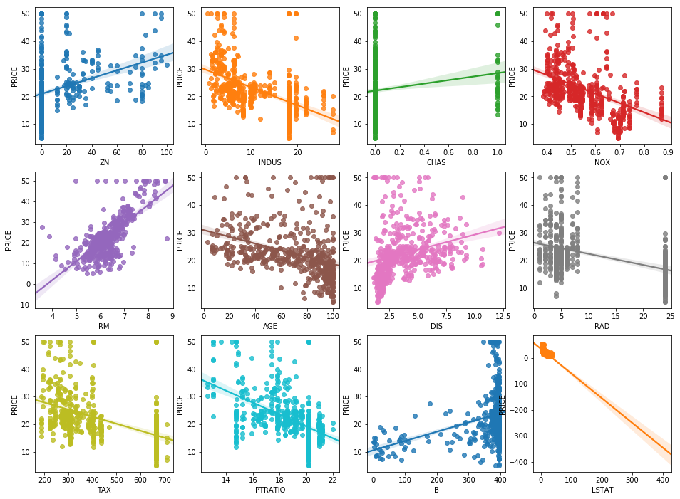
# ZN ~ LSTAT까지 각 변수들과 PRICE의 선형 관계를 sns.regplot으로 살펴보자
fix, axs = plt.subplots(figsize=(16, 12), ncols=4, nrows=3)
features = df.columns[1:-1]

for i, feature in enumerate(features):
    row = int(i/4)
    col = i%4
    sns.regplot(x=feature, y="PRICE", data=df, ax=axs[row][col])
6. 학습 및 평가 지표 살펴보기
from sklearn.model_selection import train_test_split
from sklearn.linear_model import LinearRegression
from sklearn.metrics import mean_squared_error, r2_score
y = df["PRICE"]
X = df.iloc[:,:-1]
X_train, X_test, y_train, y_test = train_test_split(X,y, test_size=0.2)
lr = LinearRegression()
lr.fit(X_train, y_train)
y_pred = lr.predict(X_test)
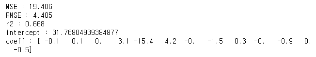
mse = mean_squared_error(y_test, y_pred)
r2 = r2_score(y_test, y_pred)
print("MSE : {0:.3f}".format(mse))
print("RMSE : {0:.3f}".format(np.sqrt(mse)))
print("r2 : {0:.3f}".format(r2))
print("intercept : {}".format(lr.intercept_))
print("coeff : {}".format(np.round(lr.coef_,1)))
7. 피처 별 회귀 계수 살펴보기
- lr.coef_를 시리즈로 만들어 정렬 후 출력
- sns.regplot에서 본대로 RM은 강한 양의 상관 관계, LSTAT은 음의 상관관계를 가짐
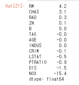
coef = pd.Series(data=np.round(lr.coef_, 1), index=X.columns)
coef.sort_values(ascending=False)
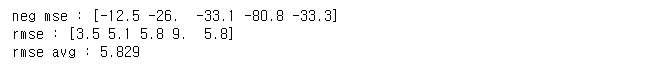
8. k fold 교차 검증 후 성능 살펴보기
from sklearn.model_selection import cross_val_score

lr = LinearRegression()

neg_mse_scores = cross_val_score(lr, X, y, scoring="neg_mean_squared_error", cv=5)
rmse = np.sqrt(-1 * neg_mse_scores)
rmse_avg = np.mean(rmse)

print("neg mse : {}".format(np.round(neg_mse_scores,1)))
print("rmse : {}".format(np.round(rmse,1)))
print("rmse avg : {0:.3f}".format(rmse_avg))'인공지능' 카테고리의 다른 글
| 파이썬머신러닝 - 21. 다항 회귀 과소 적합과 과적합 문제 (0) | 2020.12.07 |
|---|---|
| 파이썬머신러닝 - 20. 다항 회귀 (0) | 2020.12.06 |
| 파이썬머신러닝 - 18. 선형 회귀 모델과 경사 하강 법 이론과 구현 (0) | 2020.12.03 |
| 파이썬머신러닝 - 17. 스태킹 모델로 유방암 분류하기 (0) | 2020.11.30 |
| 파이썬머신러닝 - 16. 캐글 신용카드 사기 검출 (0) | 2020.11.30 |