728x90
일단 GEKKO란 라이브러리는 처음 들어보는 거지만
아까 본 영상에서 파이썬에서 GEKKO라이브러리로 역 도립진자 시뮬레이션 하는 모습을 봤었다.
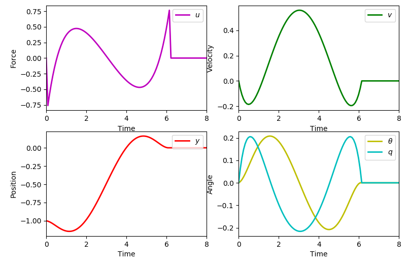
일단 코드를 가져와서 시뮬레이션 돌려보긴 했는데 결과는 이렇다.

http://apmonitor.com/do/index.php/Main/InvertedPendulum
이 자료에서는 역 도립진자시스템을 위한 제어기 모델을 설계하고 있다.
위 시연에서는 y = -1.0에서 y = 0으로 이동을 보여주고 있으며, 다른 변수 v, theta, q는 조종 전이나 조종후나 0이된다.
여기서는 역 도립진자에 대한 동역학 방정식을 정리하고 코드가 제공되고 있다.


# Contributed by Everton Colling
import matplotlib.animation as animation
import numpy as np
from gekko import GEKKO

#Defining a model
m = GEKKO()

#################################
#Weight of item
m2 = 1
#################################

#Defining the time, we will go beyond the 6.2s
#to check if the objective was achieved
m.time = np.linspace(0,8,100)
end_loc = int(100.0*6.2/8.0)

#Parameters
m1a = m.Param(value=10)
m2a = m.Param(value=m2)
final = np.zeros(len(m.time))
for i in range(len(m.time)):
    if m.time[i] < 6.2:
        final[i] = 0
    else:
        final[i] = 1
final = m.Param(value=final)

#MV
ua = m.Var(value=0)

#State Variables
theta_a = m.Var(value=0)
qa = m.Var(value=0)
ya = m.Var(value=-1)
va = m.Var(value=0)

#Intermediates
epsilon = m.Intermediate(m2a/(m1a+m2a))

#Defining the State Space Model
m.Equation(ya.dt() == va)
m.Equation(va.dt() == -epsilon*theta_a + ua)
m.Equation(theta_a.dt() == qa)
m.Equation(qa.dt() == theta_a -ua)

#Definine the Objectives
#Make all the state variables be zero at time >= 6.2
m.Obj(final*ya**2)
m.Obj(final*va**2)
m.Obj(final*theta_a**2)
m.Obj(final*qa**2)

m.fix(ya,pos=end_loc,val=0.0)
m.fix(va,pos=end_loc,val=0.0)
m.fix(theta_a,pos=end_loc,val=0.0)
m.fix(qa,pos=end_loc,val=0.0)
#Try to minimize change of MV over all horizon
m.Obj(0.001*ua**2)

m.options.IMODE = 6 #MPC
m.solve() #(disp=False)

#Plotting the results
import matplotlib.pyplot as plt
plt.figure(figsize=(12,10))

plt.subplot(221)
plt.plot(m.time,ua.value,'m',lw=2)
plt.legend([r'$u$'],loc=1)
plt.ylabel('Force')
plt.xlabel('Time')
plt.xlim(m.time[0],m.time[-1])

plt.subplot(222)
plt.plot(m.time,va.value,'g',lw=2)
plt.legend([r'$v$'],loc=1)
plt.ylabel('Velocity')
plt.xlabel('Time')
plt.xlim(m.time[0],m.time[-1])

plt.subplot(223)
plt.plot(m.time,ya.value,'r',lw=2)
plt.legend([r'$y$'],loc=1)
plt.ylabel('Position')
plt.xlabel('Time')
plt.xlim(m.time[0],m.time[-1])

plt.subplot(224)
plt.plot(m.time,theta_a.value,'y',lw=2)
plt.plot(m.time,qa.value,'c',lw=2)
plt.legend([r'$\theta$',r'$q$'],loc=1)
plt.ylabel('Angle')
plt.xlabel('Time')
plt.xlim(m.time[0],m.time[-1])

plt.rcParams['animation.html'] = 'html5'

x1 = ya.value
y1 = np.zeros(len(m.time))

#suppose that l = 1
x2 = 1*np.sin(theta_a.value)+x1
x2b = 1.05*np.sin(theta_a.value)+x1
y2 = 1*np.cos(theta_a.value)-y1
y2b = 1.05*np.cos(theta_a.value)-y1

fig = plt.figure(figsize=(8,6.4))
ax = fig.add_subplot(111,autoscale_on=False,\
                     xlim=(-1.5,0.5),ylim=(-0.4,1.2))
ax.set_xlabel('position')
ax.get_yaxis().set_visible(False)

crane_rail, = ax.plot([-1.5,0.5],[-0.2,-0.2],'k-',lw=4)
start, = ax.plot([-1,-1],[-1.5,1.5],'k:',lw=2)
objective, = ax.plot([0,0],[-0.5,1.5],'k:',lw=2)
mass1, = ax.plot([],[],linestyle='None',marker='s',\
                 markersize=40,markeredgecolor='k',\
                 color='orange',markeredgewidth=2)
mass2, = ax.plot([],[],linestyle='None',marker='o',\
                 markersize=20,markeredgecolor='k',\
                 color='orange',markeredgewidth=2)
line, = ax.plot([],[],'o-',color='orange',lw=4,\
                markersize=6,markeredgecolor='k',\
                markerfacecolor='k')
time_template = 'time = %.1fs'
time_text = ax.text(0.05,0.9,'',transform=ax.transAxes)
start_text = ax.text(-1.06,-0.3,'start',ha='right')
end_text = ax.text(0.06,-0.3,'objective',ha='left')

def init():
    mass1.set_data([],[])
    mass2.set_data([],[])
    line.set_data([],[])
    time_text.set_text('')
    return line, mass1, mass2, time_text

def animate(i):
    mass1.set_data([x1[i]],[y1[i]-0.1])
    mass2.set_data([x2b[i]],[y2b[i]])
    line.set_data([x1[i],x2[i]],[y1[i],y2[i]])
    time_text.set_text(time_template % m.time[i])
    return line, mass1, mass2, time_text

ani_a = animation.FuncAnimation(fig, animate, \
         np.arange(1,len(m.time)), \
         interval=40,blit=False,init_func=init)

# requires ffmpeg to save mp4 file
#  available from https://ffmpeg.zeranoe.com/builds/
#  add ffmpeg.exe to path such as C:\ffmpeg\bin\ in
#  environment variables

#ani_a.save('Pendulum_Control.mp4',fps=30)

plt.show()
코드는 위와 같다.
애니메이션 부분은 그렇다 치더라도 GEKKO가 뭔지 모르는 상태에선 이해하기 힘들듯 하다
개코의 소개 사이트에 들어왔다.
https://gekko.readthedocs.io/en/latest/overview.html
개코는 최대 정수, 미분 대수 방정식을 위한 최적화 소프트웨어로 선형, 이차, 비선형 그리고 최대 정수가 혼합된 프로그래밍 등 많은 범위에서 사용할수 있는 도구로, 실시간 최적화, 동역학 시뮬레이션, 비선형 예측 제어 등 모드를 제공한다고 한다.
=> 여기까지 내용을 봐서는 개코는 최적화 연산 도구로 아무래도 우리 예제에선 동역학 식을 만들어서 사용하니 이 라이브러리로 최적 계산을 수행해서 플로팅 시켜준듯하다.
일단 게코 라이브러리는 여기까지만 보자
300x250
'로봇 > 전기전자&메카' 카테고리의 다른 글
| 프로토타이핑 - 12. 아두이노 PID 튜토리얼 + PID제어기(wiki) (0) | 2020.08.16 |
|---|---|
| 프로토타이핑 - 11. GEKKO (0) | 2020.08.16 |
| 프로토타이핑 - 9. 자료 조사 1(2020.08.16) (0) | 2020.08.16 |
| 프로토타이핑 - 8. 2020.08.14 보고서 (0) | 2020.08.15 |
| 프로토타이핑 - 7. 전선 등 (0) | 2020.08.14 |